Chapter 5 Random Variables

5.1 Student Learning Objective

This section introduces some important examples of random variables. The distributions of these random variables emerge as mathematical models of real-life settings. In two of the examples the sample space is composed of integers. In the other two examples the sample space is made of continuum of values. For random variables of the latter type one may use the density, which is a type of a histogram, in order to describe the distribution.

By the end of the chapter the student should:

• Identify the Binomial, Poisson, Uniform, and Exponential random variables, relate them to real life situations, and memorize their expectations and variances.

• Relate the plot of the density/probability function and the cumulative probability function to the distribution of a random variable.

• Become familiar with the R functions that produce the density/probability of these random variables and their cumulative probabilities.

• Plot the density and the cumulative probability function of a random variable and compute probabilities associated with random variables.

5.2 Discrete Random Variables

In the previous chapter we introduced the notion of a random variable. A random variable corresponds to the outcome of an observation or a measurement prior to the actual making of the measurement. In this context one can talk of all the values that the measurement may potentially obtain. This collection of values is called the sample space. To each value in the sample space one may associate the probability of obtaining this particular value. Probabilities are like relative frequencies. All probabilities are positive and the sum of the probabilities that are associated with all the values in the sample space is equal to one.

A random variable is defined by the identification of its sample space and the probabilities that are associated with the values in the sample space. For each type of random variable we will identify first the sample space — the values it may obtain — and then describe the probabilities of the values. Examples of situations in which each type of random variable may serve as a model of a measurement will be provided. The R system provides functions for the computation of probabilities associated with specific types of random variables. We will use these functions in this and in proceeding chapters in order to carry out computations associated with the random variables and in order to plot their distributions.

The distribution of a random variable, just like the distribution of data, can be characterized using numerical summaries. For the latter we used summaries such as the mean and the sample variance and standard deviation. The mean is used to describe the central location of the distribution and the variance and standard deviation are used to characterize the total spread. Parallel summaries are used for random variable. In the case of a random variable the name expectation is used for the central location of the distribution and the variance and the standard deviation (the square root of the variation) are used to summarize the spread. In all the examples of random variables we will identify the expectation and the variance (and, thereby, also the standard deviation).

Random variables are used as probabilistic models of measurements. Theoretical considerations are used in many cases in order to define random variables and their distribution. A random variable for which the values in the sample space are separated from each other, say the values are integers, is called a discrete random variable. In this section we introduce two important integer-valued random variables: The Binomial and the Poisson random variables. These random variables may emerge as models in contexts where the measurement involves counting the number of occurrences of some phenomena.

Many other models, apart from the Binomial and Poisson, exist for discrete random variables. An example of such model, the Negative-Binomial model, will be considered in Section 5.4. Depending on the specific context that involves measurements with discrete values, one may select the Binomial, the Poisson, or one of these other models to serve as a theoretical approximation of the distribution of the measurement.

5.2.1 The Binomial Random Variable

The Binomial random variable is used in settings in which a trial that has two possible outcomes is repeated several times. Let us designate one of the outcomes as “Success” and the other as “Failure”. Assume that the probability of success in each trial is given by some number \(p\) that is larger than 0 and smaller than 1. Given a number \(n\) of repeats of the trial and given the probability of success, the actual number of trials that will produce “Success” as their outcome is a random variable. We call such random variable Binomial. The fact that a random variable \(X\) has such a distribution is marked by the expression: “\(X \sim \mathrm{Binomial}(n,p)\)”.

As an example consider tossing 10 coins. Designate “Head” as success and “Tail” as failure. For fair coins the probability of “Head” is \(1/2\). Consequently, if \(X\) is the total number of “Heads” then \(X \sim \mathrm{Binomial}(10,0.5)\), where \(n=10\) is the number of trials and \(p=0.5\) is the probability of success in each trial.

It may happen that all 10 coins turn up “Tail”. In this case \(X\) is equal to 0. It may also be the case that one of the coins turns up “Head” and the others turn up “Tail”. The random variable \(X\) will obtain the value 1 in such a case. Likewise, for any integer between 0 and 10 it may be the case that the number of “Heads” that turn up is equal to that integer with the other coins turning up “Tail”. Hence, the sample space of \(X\) is the set of integers \(\{0, 1, 2, \ldots, 10\}\). The probability of each outcome may be computed by an appropriate mathematical formula that will not be discussed here¹⁰.

The probabilities of the various possible values of a Binomial random variable may be computed with the aid of the R function “dbinom” (that uses the mathematical formula for the computation). The input to this function is a sequence of values, the value of \(n\), and the value of \(p\). The output is the sequence of probabilities associated with each of the values in the first input.

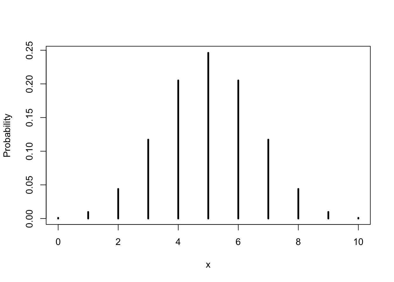
FIGURE 5.1: The Binomial(10,0.5) Distribution

For example, let us use the function in order to compute the probability that the given Binomial obtains an odd value. A sequence that contains the odd values in the Binomial sample space can be created with the expression “c(1,3,5,7,9)”. This sequence can serve as the input in the first argument of the function “dbinom”. The other arguments are “10” and “0.5”, respectively:

dbinom(c(1,3,5,7,9),10,0.5)

## [1] 0.009765625 0.117187500 0.246093750 0.117187500 0.009765625

Observe that the output of the function is a sequence of the same length as the first argument. This output contains the Binomial probabilities of the values in the first argument. In order to obtain the probability of the event \(\{\mbox{X is odd}\}\) we should sum up these probabilities, which we can do by applying the function “sum” to the output of the function that computes the Binomial probabilities:

sum(dbinom(c(1,3,5,7,9),10,0.5))

## [1] 0.5

Observe that the probability of obtaining an odd value in this specific case is equal to one half.

Another example is to compute all the probabilities of all the potential values of a \(\mathrm{Binomial}(10,0.5)\) random variable:

x <- 0:10
dbinom(x,10,0.5)

##  [1] 0.0009765625 0.0097656250 0.0439453125 0.1171875000 0.2050781250
##  [6] 0.2460937500 0.2050781250 0.1171875000 0.0439453125 0.0097656250
## [11] 0.0009765625

The expression “start.value:end.value” produces a sequence of numbers that initiate with the number “start.value” and proceeds in jumps of size one until reaching the number “end.value”. In this example, “0:10” produces the sequence of integers between 0 and 10, which is the sample space of the current Binomial example. Entering this sequence as the first argument to the function “dbinom” produces the probabilities of all the values in the sample space.

One may display the distribution of a discrete random variable with a bar plot similar to the one used to describe the distribution of data. In this plot a vertical bar representing the probability is placed above each value of the sample space. The hight of the bar is equal to the probability. A bar plot of the \(\mathrm{Binomial}(10,0.5)\) distribution is provided in Figure 5.1.

Another useful function is “pbinom”, which produces the cumulative probability of the Binomial:

pbinom(x,10,0.5)

##  [1] 0.0009765625 0.0107421875 0.0546875000 0.1718750000 0.3769531250
##  [6] 0.6230468750 0.8281250000 0.9453125000 0.9892578125 0.9990234375
## [11] 1.0000000000

cumsum(dbinom(x,10,0.5))

##  [1] 0.0009765625 0.0107421875 0.0546875000 0.1718750000 0.3769531250
##  [6] 0.6230468750 0.8281250000 0.9453125000 0.9892578125 0.9990234375
## [11] 1.0000000000

The output of the function “pbinom” is the cumulative probability \(\Prob(X \leq x)\) that the random variable is less than or equal to the input value. Observe that this cumulative probability is obtained by summing all the probabilities associated with values that are less than or equal to the input value. Specifically, the cumulative probability at \(x=3\) is obtained by the summation of the probabilities at \(x=0\), \(x=1\), \(x=2\), and \(x=3\):

\[\Prob(X \leq 3) = 0.0009765625 + 0.009765625 + 0.0439453125 + 0.1171875 = 0.171875\] The numbers in the sum are the first 4 values from the output of the function “dbinom(x,10,0.5)”, which computes the probabilities of the values of the sample space.

In principle, the expectation of the Binomial random variable, like the expectation of any other (discrete) random variable is obtained from the application of the general formulae:

\[\Expec(X) = \sum_x \big(x \times \Prob(X = x)\big)\;,\quad \Var(X) = \sum_x\big( (x-\Expec(X))^2 \times \Prob(x)\big)\;.\] However, in the specific case of the Binomial random variable, in which the probability \(\Prob(X = x)\) obeys the specific mathematical formula of the Binomial distribution, the expectation and the variance reduce to the specific formulae:

\[\Expec(X) = n p\;,\quad \Var(X) = n p(1-p)\;.\] Hence, the expectation is the product of the number of trials \(n\) with the probability of success in each trial \(p\). In the variance the number of trials is multiplied by the product of a probability of success (\(p\)) with the probability of a failure (\(1-p\)).

As illustration, let us compute for the given example the expectation and the variance according to the general formulae for the computation of the expectation and variance in random variables and compare the outcome to the specific formulae for the expectation and variance in the Binomial distribution:

X.val <- 0:10
P.val <- dbinom(X.val,10,0.5)
EX <- sum(X.val*P.val)
EX

## [1] 5

sum((X.val-EX)^2*P.val)

## [1] 2.5

This agrees with the specific formulae for Binomial variables, since \(10 \times 0.5 = 5\) and \(10 \times 0.5 \times(1-0.5) = 2.5\).

Recall that the general formula for the computation of the expectation calls for the multiplication of each value in the sample space with the probability of that value, followed by the summation of all the products. The object “X.val” contains all the values of the random variable and the object “P.val” contains the probabilities of these values. Hence, the expression “X.val*P.val” produces the product of each value of the random variable times the probability of that value. Summation of these products with the function “sum” gives the expectation, which is saved in an object that is called “EX”.

The general formula for the computation of the variance of a random variable involves the product of the squared deviation associated with each value with the probability of that value, followed by the summation of all products. The expression “(X.val-EX)^ 2” produces the sequence of squared deviations from the expectation for all the values of the random variable. Summation of the product of these squared deviations with the probabilities of the values (the outcome of “(X.val-EX)^2*P.val”) gives the variance.

When the value of \(p\) changes (without changing the number of trials \(n\)) then the probabilities that are assigned to each of the values of the sample space of the Binomial random variable change, but the sample space itself does not. For example, consider rolling a die 10 times and counting the number of times that the face 3 was obtained. Having the face 3 turning up is a “Success”. The probability \(p\) of a success in this example is 1/6, since the given face is one out of 6 equally likely faces. The resulting random variable that counts the total number of success in 10 trials has a \(\mathrm{Binomial}(10,1/6)\) distribution. The sample space is yet again equal to the set of integers \(\{0,1, \ldots,10\}\). However, the probabilities of values are different. These probabilities can again be computes with the aid of the function “dbinom”:

dbinom(x,10,1/6)

##  [1] 1.615056e-01 3.230112e-01 2.907100e-01 1.550454e-01 5.426588e-02
##  [6] 1.302381e-02 2.170635e-03 2.480726e-04 1.860544e-05 8.269086e-07
## [11] 1.653817e-08

In this case smaller values of the random variable are assigned higher probabilities and larger values are assigned lower probabilities..

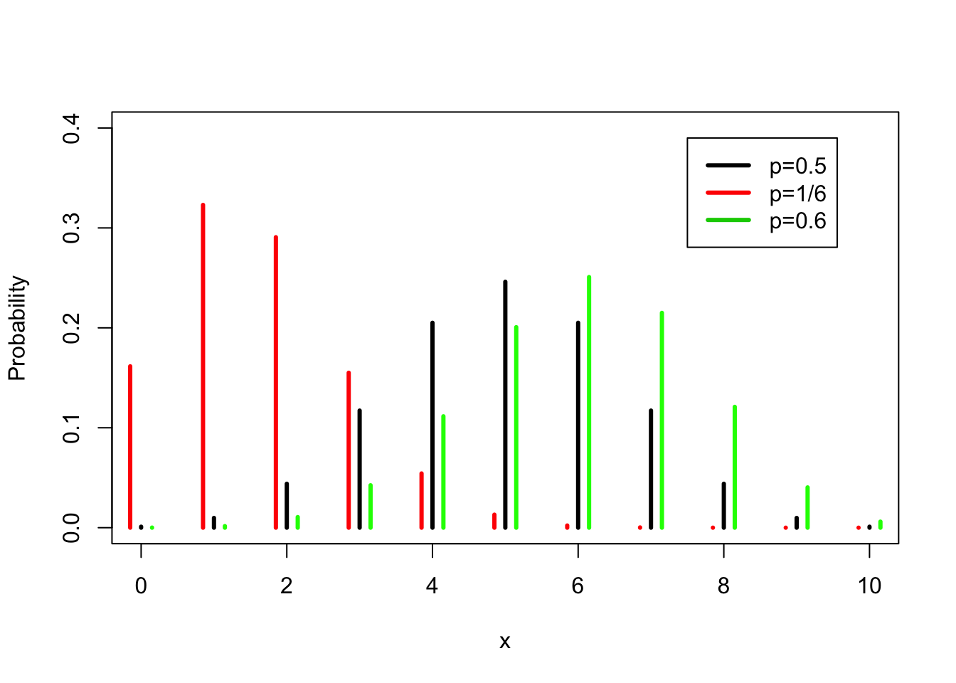
FIGURE 5.2: The Binomial Distribution for Various Probability of “Success”" \(p\)

In Figure 5.2 the probabilities for \(\mathrm{Binomial}(10,1/6)\), the \(\mathrm{Binomial}(10,1/2)\), and the \(\mathrm{Binomial}(10,0.6)\) distributions are plotted side by side. In all these 3 distributions the sample space is the same, the integers between 0 and 10. However, the probabilities of the different values differ. (Note that all bars should be placed on top of the integers. For clarity of the presentation, the bars associated with the \(\mathrm{Binomial}(10,1/6)\) are shifted slightly to the left and the bars associated with the \(\mathrm{Binomial}(10,0.6)\) are shifted slightly to the right.)

The expectation of the \(\mathrm{Binomial}(10,0.5)\) distribution is equal to \(10 \times 0.5 = 5\). Compare this to the expectation of the \(\mathrm{Binomial}(10,1/6)\) distribution, which is \(10 \times (1/6) = 1.666667\) and to the expectation of the \(\mathrm{Binomial}(10,0.6)\) distribution which equals \(10 \times 0.6 = 6\).

The variance of the \(\mathrm{Binomial}(10,0.5)\) distribution is \(10 \times 0.5 \times 0.5 = 2.5\). The variance when \(p=1/6\) is \(10 \times (1/6) \times (5/6) = 1.388889\) and the variance when \(p=0.6\) is \(10 \times 0.6 \times 0.4 = 2.4\).

Example 5.1 As an application of the Binomial distribution consider a pre-election poll. A candidate is running for office and is interested in knowing the percentage of support in the general population in its candidacy. Denote the probability of support by \(p\). In order to estimate the percentage a sample of size 300 is selected from the population. Let \(X\) be the count of supporters in the sample. A natural model for the distribution of \(X\) is the \(\mathrm{Binomial}(300,p)\) distribution, since each subject in the sample may be a supporter (“Success”) or may not be a supporter (“Failure”). The probability that a subject supports the candidate is \(p\) and there are \(n=300\) subjects in the sample.

Example 5.2 As another example consider the procedure for quality control that is described in Discussion Forum of Chapter 4. According to the procedure 20 items are tested and the number of faulty items is recorded. If \(p\) is the probability that an item is identified as faulty then the distribution of the total number of faulty items may be modeled by the \(\mathrm{Binomial}(20,p)\) distribution.

In both examples one may be interested in making statements on the probability \(p\) based on the sample. Statistical inference relates the actual count obtained in the sample to the theoretical Binomial distribution in order to make such statements.

5.2.2 The Poisson Random Variable

The Poisson distribution is used as an approximation of the total number of occurrences of rare events. Consider, for example, the Binomial setting that involves \(n\) trials with \(p\) as the probability of success of each trial. Then, if \(p\) is small but \(n\) is large then the number of successes \(X\) has, approximately, the Poisson distribution.

The sample space of the Poisson random variable is the unbounded collection of integers: \(\{0,1,2, \ldots\}\). Any integer value is assigned a positive probability. Hence, the Poisson random variable is a convenient model when the maximal number of occurrences of the events in a-priori unknown or is very large. For example, one may use the Poisson distribution to model the number of phone calls that enter a switchboard in a given interval of time or the number of malfunctioning components in a shipment of some product.

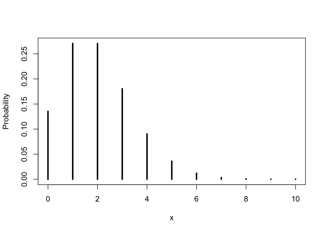
FIGURE 5.3: The Poisson(2) Distribution

The Binomial distribution was specified by the number of trials \(n\) and probability of success in each trial \(p\). The Poisson distribution is specified by its expectation, which we denote by \(\lambda\). The expression “\(X \sim \mathrm{Poisson}(\lambda)\)” states that the random variable \(X\) has a Poisson distribution¹¹ with expectation \(\Expec(X) = \lambda\). The function “dpois” computes the probability, according to the Poisson distribution, of values that are entered as the first argument to the function. The expectation of the distribution is entered in the second argument. The function “ppois” computes the cumulative probability. Consequently, we can compute the probabilities and the cumulative probabilities of the values between 0 and 10 for the \(\mathrm{Poisson}(2)\) distribution via:

x <- 0:10
dpois(x,2)

##  [1] 1.353353e-01 2.706706e-01 2.706706e-01 1.804470e-01 9.022352e-02
##  [6] 3.608941e-02 1.202980e-02 3.437087e-03 8.592716e-04 1.909493e-04
## [11] 3.818985e-05

ppois(x,2)

##  [1] 0.1353353 0.4060058 0.6766764 0.8571235 0.9473470 0.9834364 0.9954662
##  [8] 0.9989033 0.9997626 0.9999535 0.9999917

The probability function of the Poisson distribution with \(\lambda = 2\), in the range between 0 and 10, is plotted in Figure 5.3. Observe that in this example probabilities of the values 8 and beyond are very small. As a matter of fact, the cumulative probability at \(x=7\) (the 8th value in the output of “ppois(x,2)”) is approximately 0.999, out of the total cumulative probability of 1.000, leaving a total probability of about 0.001 to be distributed among all the values larger than 7.

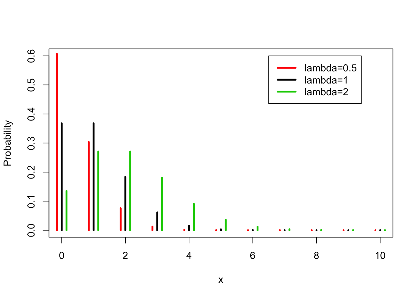
FIGURE 5.4: The Poisson Distribution for Various Values of \(\lambda\)

Let us compute the expectation of the given Poisson distribution:

X.val <- 0:10
P.val <- dpois(X.val,2)
sum(X.val*P.val)

## [1] 1.999907

Observe that the outcome is almost, but not quite, equal to \(2.00\), which is the actual value of the expectation. The reason for the inaccuracy is the fact that we have based the computation in R on the first 11 values of the distribution only, instead of the infinite sequence of values. A more accurate result may be obtained by the consideration of the first 101 values:

X.val <- 0:100
P.val <- dpois(X.val,2)
EX <- sum(X.val*P.val)
EX

## [1] 2

sum((X.val-EX)^2*P.val)

## [1] 2

In the last expression we have computed the variance of the Poisson distribution and obtained that it is equal to the expectation. This results can be validated mathematically. For the Poisson distribution it is always the case that the variance is equal to the expectation, namely to \(\lambda\): \[\Expec(X) = \Var(X) = \lambda\;.\]

In Figure 5.4 you may find the probabilities of the Poisson distribution for \(\lambda = 0.5\), \(\lambda = 1\) and \(\lambda = 2\). Notice once more that the sample space is the same for all the Poisson distributions. What varies when we change the value of \(\lambda\) are the probabilities. Observe that as \(\lambda\) increases then probability of larger values increases as well.

Example 5.3 A radio active element decays by the release of subatomic particles and energy. The decay activity is measured in terms of the number of decays per second in a unit mass. A typical model for the distribution of the number of decays is the Poisson distribution. Observe that the number of decays in a second is a integer and, in principle, it may obtain any integer value larger or equal to zero. The event of a radio active decay of an atom is a relatively rare event. Therefore, the Poisson model is likely to fit this phenomena¹².

Example 5.4 Consider an overhead power line suspended between two utility poles. During rain, drops of water may hit the power line. The total number of drops that hit the line in a one minute period may be modeled by a Poisson random variable.

5.3 Continuous Random Variable

Many types of measurements, such as height, weight, angle, temperature, etc., may in principle have a continuum of possible values. Continuous random variables are used to model uncertainty regarding future values of such measurements.

The main difference between discrete random variables, which is the type we examined thus far, and continuous random variable, that are added now to the list, is in the sample space, i.e., the collection of possible outcomes. The former type is used when the possible outcomes are separated from each other as the integers are. The latter type is used when the possible outcomes are the entire line of real numbers or when they form an interval (possibly an open ended one) of real numbers.

The difference between the two types of sample spaces implies differences in the way the distribution of the random variables is being described. For discrete random variables one may list the probability associated with each value in the sample space using a table, a formula, or a bar plot. For continuous random variables, on the other hand, probabilities are assigned to intervals of values, and not to specific values. Thence, densities are used in order to display the distribution.

Densities are similar to histograms, with areas under the plot corresponding to probabilities. We will provide a more detailed description of densities as we discuss the different examples of continuous random variables.

In continuous random variables integration replaces summation and the density replaces the probability in the computation of quantities such as the probability of an event, the expectation, and the variance.

Hence, if the expectation of a discrete random variable is given in the formula \(\Expec(X) = \sum_x \big(x \times \Prob(x)\big)\), which involves the summation over all values of the product between the value and the probability of the value, then for continuous random variable the definition becomes:

\[\Expec(X) = \int \big(x \times f(x)\big)dx\;,\] where \(f(x)\) is the density of \(X\) at the value \(x\). Therefore, in the expectation of a continuous random variable one multiplies the value by the density at the value. This product is then integrated over the sample space.

Likewise, the formula \(\Var(X) = \sum_x\big( (x-\Expec(X))^2 \times \Prob(x)\big)\) for the variance is replaced by:

\[\Var(X) =\int\big((x-\Expec(X))^2 \times f(x) \big) dx\;.\] Nonetheless, the intuitive interpretation of the expectation as the central value of the distribution that identifies the location and the interpretation of the standard deviation (the square root of the variance) as the summary of the total spread of the distribution is still valid.

In this section we will describe two types of continuous random variables: Uniform and Exponential. In the next chapter another example – the Normal distribution – will be introduced.

5.3.1 The Uniform Random Variable

The Uniform distribution is used in order to model measurements that may have values in a given interval, with all values in this interval equally likely to occur.

For example, consider a random variable \(X\) with the Uniform distribution over the interval \([3,7]\), denoted by “\(X \sim \mathrm{Uniform}(3,7)\)”. The density function at given values may be computed with the aid of the function “dunif”. For instance let us compute the density of the \(\mathrm{Uniform}(3,7)\) distribution over the integers \(\{0, 1, \ldots, 10\}\):

dunif(0:10,3,7)

##  [1] 0.00 0.00 0.00 0.25 0.25 0.25 0.25 0.25 0.00 0.00 0.00

Notice that for the values 0, 1, and 2, and the values 8, 9 and 10 that are outside of the interval the density is equal to zero, indicating that such values cannot occur in the given distribution. The values of the density at integers inside the interval are positive and equal to each other. The density is not restricted to integer values. For example, at the point \(4.73\) we get that the density is positive and of the same height:

dunif(4.73,3,7)

## [1] 0.25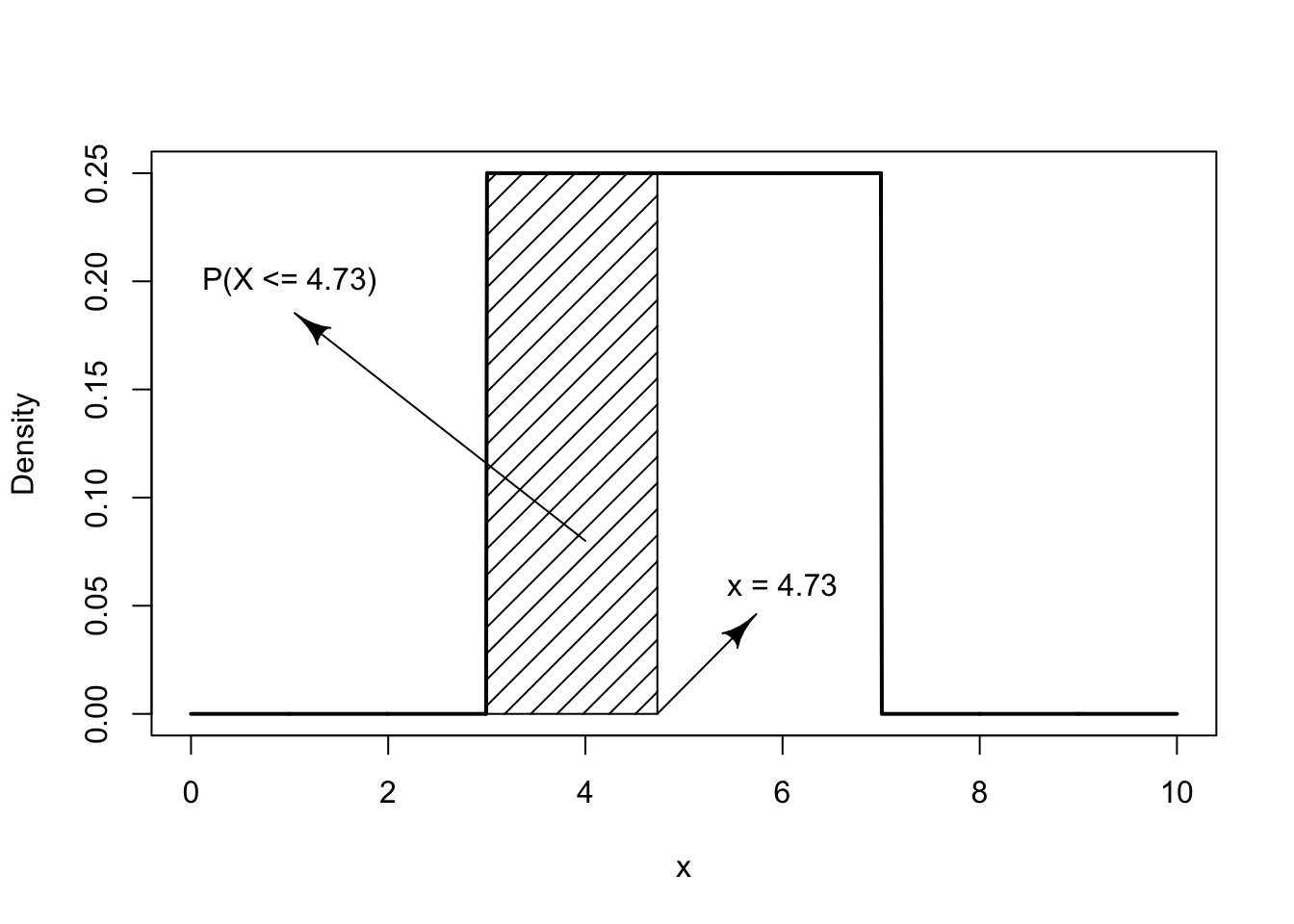

FIGURE 5.5: The Uniform(3,7) Distribution

A plot of the \(\mathrm{Uniform}(3,7)\) density is given in Figure 5.5 in the form of a solid line. Observe that the density is positive over the interval \([3,7]\) where its height is 1/4. Area under the curve in the density corresponds to probability. Indeed, the fact that the total probability is one is reflected in the total area under the curve being equal to 1. Over the interval \([3,7]\) the density forms a rectangle. The base of the rectangle is the length of the interval \(7-3=4\). The height of the rectangle is thus equal to 1/4 in order to produce a total area of \(4 \times (1/4) = 1\).

The function “punif” computes the cumulative probability of the uniform distribution. The probability \(\Prob(X \leq 4.73)\), for \(X \sim \mathrm{Uniform}(3,7)\), is given by:

punif(4.73,3,7)

## [1] 0.4325

This probability corresponds to the marked area to the left of the point \(x = 4.73\) in Figure 5.5. This area of the marked rectangle is equal to the length of the base 4.73 - 3 = 1.73, times the height of the rectangle 1/(7-3) = 1/4. Indeed:

(4.73-3)/(7-3)

## [1] 0.4325

is the area of the marked rectangle and is equal to the probability.

Let us use R in order to plot the density and the cumulative probability functions of the Uniform distribution. We produce first a large number of points in the region we want to plot. The points are produced with aid of the function “seq”. The output of this function is a sequence with equally spaced values. The starting value of the sequence is the first argument in the input of the function and the last value is the second argument in the input. The argument “length=1000” sets the length of the sequence, 1,000 values in this case:

x <- seq(0,10,length=1000)
den <- dunif(x,3,7)
plot(x,den)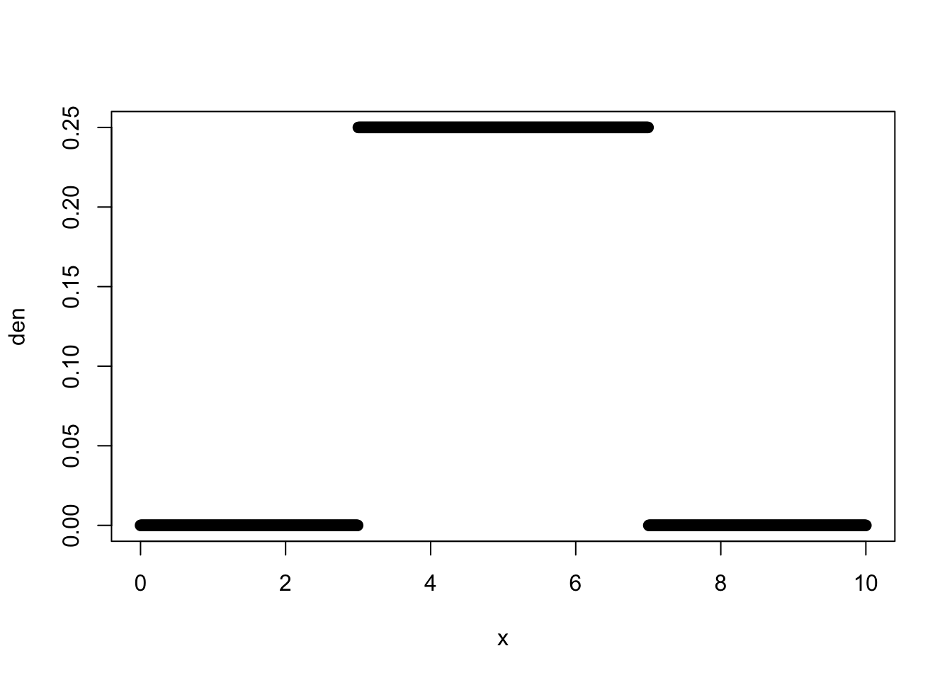

The object “den” is a sequence of length 1,000 that contains the density of the \(\mathrm{Uniform}(3,7)\) evaluated over the values of “x”. When we apply the function “plot” to the two sequences we get a scatter plot of the 1,000 points.

A scatter plot is a plot of points. Each point in the scatter plot is identify by its horizontal location on the plot (its “\(x\)” value) and by its vertical location on the plot (its \(y\) value). The horizontal value of each point in the plot is determined by the first argument to the function “plot” and the vertical value is determined by the second argument. For example, the first value in the sequence “x” is 0. The value of the Uniform density at this point is 0. Hence, the first value of the sequence “den” is also 0. A point that corresponds to these values is produced in the plot. The horizontal value of the point is 0 and the vertical value is 0. In a similar way the other 999 points are plotted. The last point to be plotted has a horizontal value of 10 and a vertical value of 0.

The number of points that are plotted is large and they overlap each other in the graph and thus produce an impression of a continuum. In order to obtain nicer looking plots we may choose to connect the points to each other with segments and use smaller points. This may be achieved by the addition of the argument “type=l”, with the letter l for line, to the plotting function:

plot(x,den,type="l")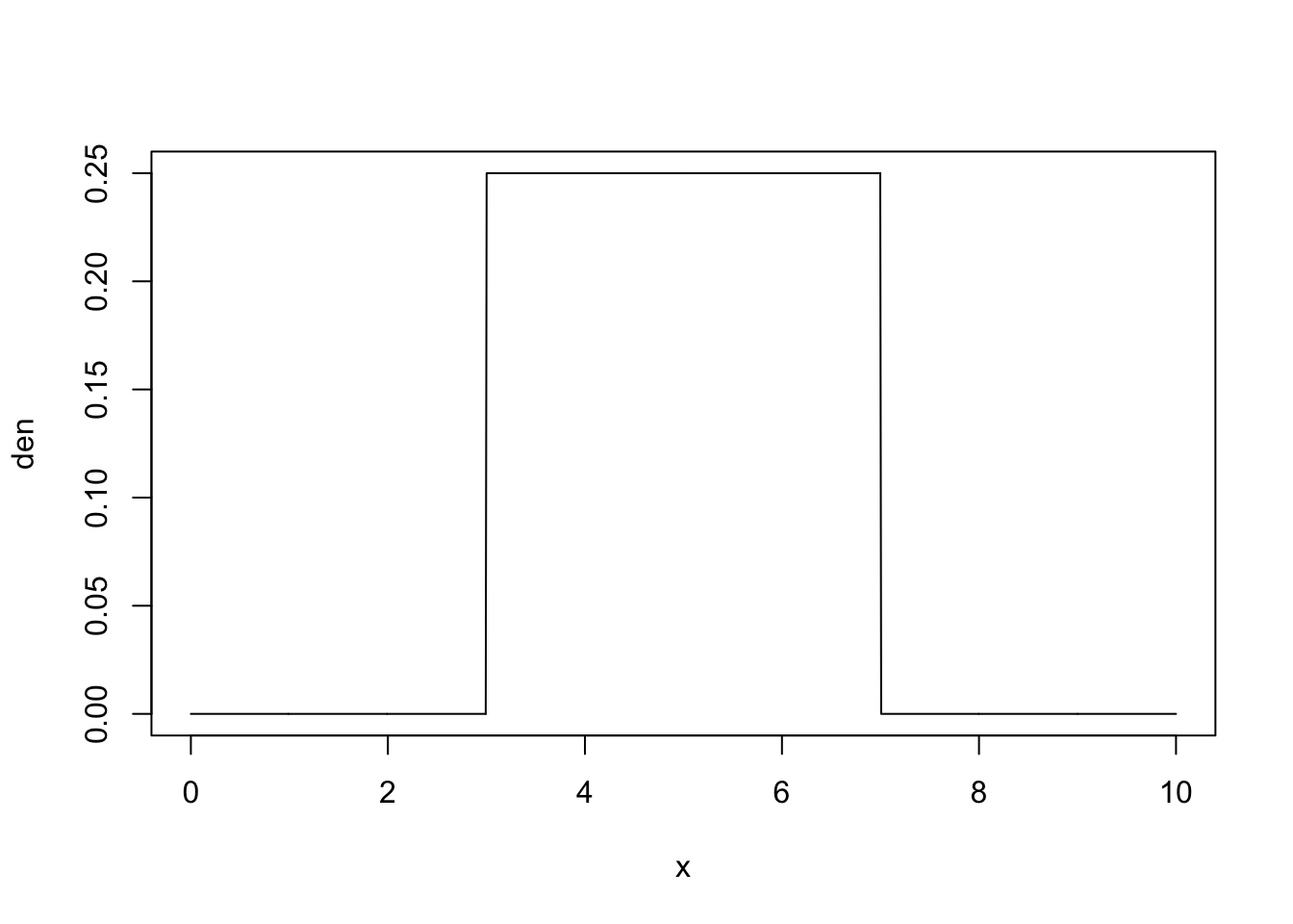

The cumulative probability of the \(\mathrm{Uniform}(3,7)\) is produced by the code:

cdf <- punif(x,3,7)
plot(x,cdf,type="l")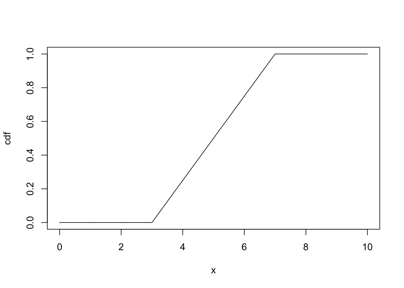

One can think of the density of the Uniform as an histogram¹³. The expectation of a Uniform random variable is the middle point of it’s histogram. Hence, if \(X \sim \mathrm{Uniform}(a,b)\) then:

\[\Expec(X) = \frac{a+b}{2}\;.\] For the \(X \sim \mathrm{Uniform}(3,7)\) distribution the expectation is \(\Expec(X)= (3+7)/2 = 5\). Observe that 5 is the center of the Uniform density in Plot 5.5.

It can be shown that the variance of the \(\mathrm{Uniform}(a,b)\) is equal to

\[\Var(X) = \frac{(b-a)^2}{12}\;,\] with the standard deviation being the square root of this value. Specifically, for \(X \sim \mathrm{Uniform}(3,7)\) we get that \(\Var(X) = (7-3)^2/12 = 1.333333\). The standard deviation is equal to \(\sqrt{1.333333} = 1.154701\).

Example 5.5 In Example 5.4 we considered rain drops that hit an overhead power line suspended between two utility poles. The number of drops that hit the line can be modeled using the Poisson distribution. The position between the two poles where a rain drop hits the line can be modeled by the Uniform distribution. The rain drop can hit any position between the two utility poles. Hitting one position along the line is as likely as hitting any other position.

Example 5.6 Meiosis is the process in which a diploid cell that contains two copies of the genetic material produces an haploid cell with only one copy (sperms or eggs, depending on the sex). The resulting molecule of genetic material is linear molecule (chromosome) that is composed of consecutive segments: a segment that originated from one of the two copies followed by a segment from the other copy and vice versa. The border points between segments are called points of crossover. The Haldane model for crossovers states that the position of a crossover between two given loci on the chromosome corresponds to the Uniform distribution and the total number of crossovers between these two loci corresponds to the Poisson distribution.

5.3.2 The Exponential Random Variable

The Exponential distribution is frequently used to model times between events. For example, times between incoming phone calls, the time until a component becomes malfunction, etc. We denote the Exponential distribution via “\(X \sim \mathrm{Exponential}(\lambda)\)”, where \(\lambda\) is a parameter that characterizes the distribution and is called the rate of the distribution. The overlap between the parameter used to characterize the Exponential distribution and the one used for the Poisson distribution is deliberate. The two distributions are tightly interconnected. As a matter of fact, it can be shown that if the distribution between occurrences of a phenomena has the Exponential distribution with rate \(\lambda\) then the total number of the occurrences of the phenomena within a unit interval of time has a \(\mathrm{Poisson}(\lambda)\) distribution.

The sample space of an Exponential random variable contains all non-negative numbers. Consider, for example, \(X \sim \mathrm{Exponential}(0.5)\). The density of the distribution in the range between 0 and 10 is presented in Figure 5.6. Observe that in the Exponential distribution smaller values are more likely to occur in comparison to larger values. This is indicated by the density being larger at the vicinity of 0. The density of the exponential distribution given in the plot is positive, but hardly so, for values larger than 10.

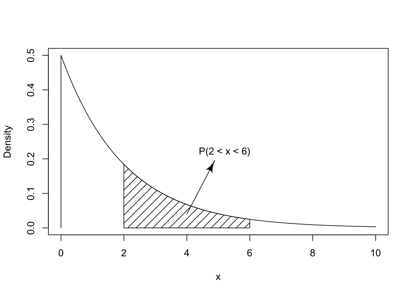
FIGURE 5.6: The Exponential(0.5) Distribution

The density of the Exponential distribution can be computed with the aid of the function “dexp”¹⁴. The cumulative probability can be computed with the function “pexp”. For illustration, assume \(X \sim \mathrm{Exponential}(0.5)\). Say one is interested in the computation of the probability \(\Prob(2 < X \leq 6)\) that the random variable obtains a value that belongs to the interval \((2,6]\). The required probability is indicated as the marked area in Figure 5.6. This area can be computed as the difference between the probability \(\Prob(X \leq 6)\), the area to the left of 6, and the probability \(\Prob(X \leq 2)\), the area to the left of 2:

pexp(6,0.5) - pexp(2,0.5)

## [1] 0.3180924

The difference is the probability of belonging to the interval, namely the area marked in the plot.

The expectation of \(X\), when \(X \sim \mathrm{Exponential}(\lambda)\), is given by the equation:

\[\Expec(X) = 1/\lambda\;,\] and the variance is given by:

\[\Var(X) =1/\lambda^2\;.\] The standard deviation is the square root of the variance, namely \(1/\lambda\). Observe that the larger is the rate the smaller are the expectation and the standard deviation.

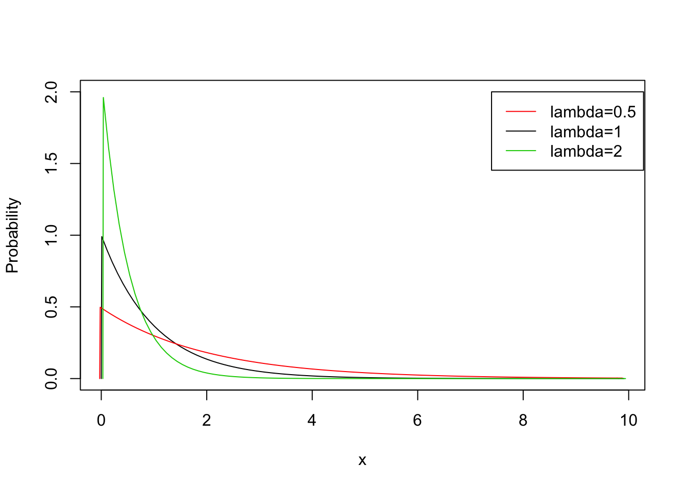
FIGURE 5.7: The Exponential Distribution for Various Values of \(\lambda\)

In Figure 5.7 the densities of the Exponential distribution are plotted for \(\lambda = 0.5\), \(\lambda = 1\), and \(\lambda = 2\). Notice that with the increase in the value of the parameter then the values of the random variable tends to become smaller. This inverse relation makes sense in connection to the Poisson distribution. Recall that the Poisson distribution corresponds to the total number of occurrences in a unit interval of time when the time between occurrences has an Exponential distribution. A larger expectation \(\lambda\) of the Poisson corresponds to a larger number of occurrences that are likely to take place during the unit interval of time. The larger is the number of occurrences the smaller are the time intervals between occurrences.

Example 5.7 Consider Examples 5.4 and 5.5 that deal with rain dropping on a power line. The times between consecutive hits of the line may be modeled by the Exponential distribution. Hence, the time to the first hit has an Exponential distribution. The time between the first and the second hit is also Exponentially distributed, and so on.

Example 5.8 Return to Example 5.3 that deals with the radio activity of some element. The total count of decays per second is model by the Poisson distribution. The times between radio active decays is modeled according to the Exponential distribution. The rate \(\lambda\) of that Exponential distribution is equal to the expectation of the total count of decays in one second, i.e. the expectation of the Poisson distribution.

5.4 Exercises

Exercise 5.1 A particular measles vaccine produces a reaction (a fever higher that 102 Fahrenheit) in each vaccinee with probability of 0.09. A clinic vaccinates 500 people each day.

1. What is the expected number of people that will develop a reaction each day?

2. What is the standard deviation of the number of people that will develop a reaction each day?

3. In a given day, what is the probability that more than 40 people will develop a reaction?

4. In a given day, what is the probability that the number of people that will develop a reaction is between 50 and 45 (inclusive)?

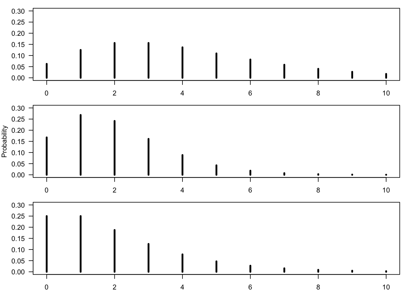
FIGURE 5.8: Bar Plots of the Negative-Binomial Distribution

Exercise 5.2 The Negative-Binomial distribution is yet another example of a discrete, integer valued, random variable. The sample space of the distribution are all non-negative integers \(\{0, 1, 2, \ldots\}\). The fact that a random variable \(X\) has this distribution is marked by “\(X \sim \mbox{Negative-Binomial}(r,p)\)”, where \(r\) and \(p\) are parameters that specify the distribution.

Consider 3 random variables from the Negative-Binomial distribution:

• \(X_1 \sim \mbox{Negative-Binomial}(2,0.5)\)

• \(X_2 \sim \mbox{Negative-Binomial}(4,0.5)\)

• \(X_3 \sim \mbox{Negative-Binomial}(8,0.8)\)

The bar plots of these random variables are presented in Figure 5.8, re-organizer in a random order.

1. Produce bar plots of the distributions of the random variables \(X_1\), \(X_2\), \(X_3\) in the range of integers between 0 and 15 and thereby identify the pair of parameters that produced each one of the plots in Figure 5.8. Notice that the bar plots can be produced with the aid of the function “plot” and the function “dnbinom(x,r,p)”, where “x” is a sequence of integers and “r” and “p” are the parameters of the distribution. Pay attention to the fact that you should use the argument “type = h” in the function “plot” in order to produce the horizontal bars.

2. Below is a list of pairs that includes an expectation and a variance. Each of the pairs is associated with one of the random variables \(X_1\), \(X_2\), and \(X_3\):

   1. \(\Expec(X) = 4\), \(\Var(X) = 8\).

   2. \(\Expec(X) = 2\), \(\Var(X) = 4\).

   3. \(\Expec(X) = 2\), \(\Var(X) = 2.5\).

   Use Figure 5.8 in order to match the random variable with its associated pair. Do not use numerical computations or formulae for the expectation and the variance in the Negative-Binomial distribution in order to carry out the matching¹⁵. Use, instead, the structure of the bar-plots.

5.5 Summary

Glossary

Binomial Random Variable:

The number of successes among \(n\) repeats of independent trials with a probability \(p\) of success in each trial. The distribution is marked as \(\mathrm{Binomial}(n,p)\).

Poisson Random Variable:

An approximation to the number of occurrences of a rare event, when the expected number of events is \(\lambda\). The distribution is marked as \(\mathrm{Poisson}(\lambda)\).

Density:

Histogram that describes the distribution of a continuous random variable. The area under the curve corresponds to probability.

Uniform Random Variable:

A model for a measurement with equally likely outcomes over an interval \([a,b]\). The distribution is marked as \(\mathrm{Uniform}(a,b)\).

Exponential Random Variable:

A model for times between events. The distribution is marked as \(\mathrm{Exponential}(\lambda)\).

Discuss in the Forum

This unit deals with two types of discrete random variables, the Binomial and the Poisson, and two types of continuous random variables, the Uniform and the Exponential. Depending on the context, these types of random variables may serve as theoretical models of the uncertainty associated with the outcome of a measurement.

In your opinion, is it or is it not useful to have a theoretical model for a situation that occurs in real life?

When forming your answer to this question you may give an example of a situation from you own field of interest for which a random variable, possibly from one of the types that are presented in this unit, can serve as a model. Discuss the importance (or lack thereof) of having a theoretical model for the situation.

For example, the Exponential distribution may serve as a model for the time until an atom of a radio active element decays by the release of subatomic particles and energy. The decay activity is measured in terms of the number of decays per second. This number is modeled as having a Poisson distribution. Its expectation is the rate of the Exponential distribution. For the radioactive element Carbon-14 (\({}^{\mbox{\tiny 14}}\mathrm{C}\)) the decay rate is \(3.8394 \times 10^{-12}\) particles per second. Computations that are based on the Exponential model may be used in order to date ancient specimens.

Summary of Formulas

Discrete Random Variable:

\[\begin{aligned} \Expec(X) &= \sum_x \big(x \times \Prob(x)\big) \\ \Var(X) &= \sum_x\big( (x-\Expec(X))^2 \times \Prob(x)\big) \end{aligned}\]

Continuous Random Variable:

\[\begin{aligned} \Expec(X) &= \int \big(x \times f(x)\big)dx \\ \Var(X) &= \int\big((x-\Expec(X))^2 \times f(x) \big) dx \end{aligned}\]

Binomial:

\(\Expec(X) = n p \;, \quad \Var(X) = n p(1-p)\)

Poisson:

\(\Expec(X) = \lambda\;, \quad \Var(X) = \lambda\)

Uniform:

\(\Expec(X) = (a+b)/2\;, \quad \Var(X)= (b-a)^2/12\)

Exponential:

\(\Expec(X) = 1/\lambda\;, \quad \Var(X)= 1/\lambda^2\)

---

10. If \(X\sim \mathrm{Binomial}(n,p)\) then \(\Prob(X = x) = {n \choose x} p^x (1-p)^{n-x}\), for \(x = 0, 1, \ldots, n\).↩

11. If \(X \sim \mathrm{Poisson}(\lambda)\) then \(\Prob(X=x) = e^{-\lambda}\lambda^x/x!\), for \(x=0,1,2,\ldots\).↩

12. The number of decays may also be considered in the \(\mathrm{Binomial}(n,p)\) setting. The number \(n\) is the total number of atoms in the unit mass and \(p\) is the probability that an atom decays within the given second. However, since \(n\) is very large and \(p\) is very small we get that the Poisson distribution is an appropriate model for the count.↩

13. If \(X \sim \mathrm{Uniform}(a,b)\) then the density is \(f(x) = 1/(b-a)\), for \(a \leq x \leq b\), and it is equal to 0 for other values of \(x\).↩

14. If \(X \sim \mathrm{Exponential}(\lambda)\) then the density is \(f(x) =\lambda e^{-\lambda x}\), for \(0 \leq x\), and it is equal to 0 for \(x < 0\).↩

15. It can be shown, or else found on the web, that if \(X\sim \mbox{Negative-Binomial}(r,p)\) then \(\Expec(X) = r(1-p)/p\) and \(\Var(X) = r(1-p)/p^2\).↩