Chapter 11 Confidence Intervals

11.1 Student Learning Objectives

A confidence interval is an estimate of an unknown parameter by a range of values. This range contains the value of the parameter with a prescribed probability, called the confidence level. In this chapter we discuss the construction of confidence intervals for the expectation and for the variance of a measurement as well as for the probability of an event. In some cases the construction will apply the Normal approximation suggested by the Central Limit Theorem. This approximation is valid when the sample size is large enough. The construction of confidence intervals for a small sample is considered in the context of Normal measurements. By the end of this chapter, the student should be able to:

• Define confidence intervals and confidence levels.

• Construct a confidence interval for the expectation of a measurement and for the probability of an event.

• Construct a confidence interval for expectation and for the variance of a Normal measurement.

• Compute the sample size that will produce a confidence interval of a given width.

11.2 Intervals for Mean and Proportion

A confidence interval, like a point estimator, is a method for estimating the unknown value of a parameter. However, instead of producing a single number, the confidence interval is an interval of numbers. The interval of values is calculated from the data. The confidence interval is likely to include the unknown population parameter. The probability of the event of inclusion is denoted as the confidence level of the confidence intervals.

This section presents a method for the computation of confidence intervals for the expectation of a measurement and a similar method for the computation of a confidence interval for the probability of an event. These methods rely on the application of the Central Limit Theorem to the sample average in the one case, and to the sample proportion in the other case.

In the first subsection we compute a confidence interval for the expectation of the variable “price” and a confidence interval for the proportion of diesel cars. The confidence intervals are computed based on the data in the file “cars.csv”. In the subsequent subsections we discuss the theory behind the computation of the confidence intervals and explain the meaning of the confidence level. Subsection 11.2.2 does so with respect to the confidence interval for the expectation and Subsection 11.2.3 with respect to the confidence interval for the proportion.

11.2.1 Examples of Confidence Intervals

A point estimator of the expectation of a measurement is the sample average of the variable that is associated with the measurement. A confidence interval is an interval of numbers that is likely to contain the parameter value. A natural interval to consider is an interval centered at the sample average \(\bar x\). The interval is set to have a width that assures the inclusion of the parameter value in the prescribed probability, namely the confidence level.

Consider the confidence interval for the expectation. The structure of the confidence interval of confidence level 95% is \([\bar x - 1.96 \cdot s/\sqrt{n}, \bar x + 1.96 \cdot s/\sqrt{n}]\), where \(s\) is the estimated standard deviation of the measurement (namely, the sample standard deviation) and \(n\) is the sample size. This interval may be expressed in the form:

\[\bar x \pm 1.96 \cdot s/\sqrt{n}\;.\]

As an illustration, let us construct a 0.95-confidence interval for the expected price of a car. :

cars <- read.csv("_data/cars.csv")
x.bar <- mean(cars$price,na.rm=TRUE)
s <- sd(cars$price,na.rm=TRUE)
n <- 201

In the first line of code the data in the file “cars.csv” is stored in a data frame called “cars”. In the second line the average \(\bar x\) is computed for the variable “price” in the data frame “cars”. This average is stored under the name “x.bar”. Recall that the variable “price” contains 4 missing values. Hence, in order to compute the average of the non-missing values we should set a “TRUE” value to the argument “na.rm”. The sample standard deviation “s” is computed in the third line by the application of the function “sd”. We set once more the argument “na.rm=TRUE” in order to deal with the missing values. Finally, in the last line we store the sample size “n”, the number of non-missing values.

Let us compute the lower and the upper limits of the confidence interval for the expectation of the price:

x.bar - 1.96*s/sqrt(n)

## [1] 12108.47

x.bar + 1.96*s/sqrt(n)

## [1] 14305.79

The lower limit of the confidence interval turns out to be $12,108.47 and the upper limit is $14,305.79. The confidence interval is the range of values between these two numbers.

Consider, next, a confidence interval for the probability of an event. The estimate of the probability \(p\) is \(\hat p\), the relative proportion of occurrences of the event in the sample. Again, we construct an interval about this estimate. In this case, a confidence interval of confidence level 95% is of the form \(\big[\hat p - 1.96 \cdot \sqrt{\hat p(1-\hat p)/n}, \hat p + 1.96 \cdot \sqrt{\hat p(1-\hat p)/n}\big]\), where \(n\) is the sample size. Observe that \(\hat p\) replaces \(\bar x\) as the estimate of the parameter and that \(\hat p(1-\hat p)/n\) replace \(s^2/n\) as the estimate of the variance of the estimator. The confidence interval for the probability may be expressed in the form:

\[\hat p \pm 1.96 \cdot \sqrt{\hat p (1-\hat p)/n}\;.\]

As an example, let us construct a confidence interval for the proportion of car types that use diesel fuel. The variable “fuel.type” is a factor that records the type of fuel the car uses, either diesel or gas:

table(cars$fuel.type)

## 
## diesel    gas 
##     20    185

Only 20 of the 205 types of cars are run on diesel in this data set. The point estimation of the probability of such car types and the confidence interval for this probability are:

n <- 205
p.hat <- 20/n
p.hat

## [1] 0.09756098

p.hat - 1.96*sqrt(p.hat*(1-p.hat)/n)

## [1] 0.05694226

p.hat + 1.96*sqrt(p.hat*(1-p.hat)/n)

## [1] 0.1381797

The point estimation of the probability is \(\hat p = 20/205 \approx 0.098\) and the confidence interval, after rounding up, is \([0.057, 0.138]\).

11.2.2 Confidence Intervals for the Mean

In the previous subsection we computed a confidence interval for the expected price of a car and a confidence interval for the probability that a car runs on diesel. In this subsection we explain the theory behind the construction of confidence intervals for the expectation. The theory provides insight to the way confidence intervals should be interpreted. In the next subsection we will discuss the theory behind the construction of confidence intervals for the probability of an event.

Assume one is interested in a confidence interval for the expectation of a measurement \(X\). For a sample of size \(n\), one may compute the sample average \(\bar X\), which is the point estimator for the expectation. The expected value of the sample average is the expectation \(\Expec(X)\), for which we are trying to produce the confidence interval. Moreover, the variance of the sample average is \(\Var(X)/n\), where \(\Var(X)\) is the variance of a single measurement and \(n\) is the sample size.

The construction of a confidence interval for the expectation relies on the Central Limit Theorem and on estimation of the variance of the measurement. The Central Limit Theorem states that the distribution of the (standardized) sample average \(Z = (\bar X - \Expec(X)/\sqrt{\Var(X)/n}\) is approximately standard Normal for a large enough sample size. The variance of the measurement can be estimated using the sample variance \(S^2\).

Supposed that we are interested in a confidence interval with a confidence level of 95%. The value 1.96 is the 0.975-percentile of the standard Normal. Therefore, about 95% of the distribution of the standardized sample average is concentrated in the range \([-1.96,1,96]\):

\[\Prob \bigg(\bigg|\frac{\bar X - \Expec(X)}{\sqrt{\Var(X)/n}}\bigg| \leq 1.96 \bigg) \approx 0.95\]

The event, the probability of which is being described in the last display, states that the absolute value of deviation of the sample average from the expectation, divided by the standard deviation of the sample average, is no more than 1.96. In other words, the distance between the sample average and the expectation is at most 1.96 units of standard deviation. One may rewrite this event in a form that puts the expectation within an interval that is centered at the sample average⁴⁶:

\[\begin{aligned} \Big\{|\bar X - \Expec(X)| \leq 1.96 \cdot \sqrt{\Var(X)/n} \Big\} \quad \Longleftrightarrow & \\ \Big\{ \bar X -1.96 \cdot\sqrt{\Var(X)/n} \leq \Expec(X) &\leq \bar X + 1.96 \cdot \sqrt{\Var(X)/n}\Big\}\;.\end{aligned}\]

Clearly, the probability of the later event is (approximately) 0.95 since we are considering the same event, each time represented in a different form. The second representation states that the expectation \(\Expec(X)\) belongs to an interval about the sample average: \(\bar X \pm 1.96 \sqrt{\Var(X)/n}\). This interval is, almost, the confidence interval we seek.

The difficulty is that we do not know the value of the variance \(\Var(X)\), hence we cannot compute the interval in the proposed form from the data. In order to overcome this difficulty we recall that the unknown variance may nonetheless be estimated from the data:

\[S^2 \approx \Var(X) \quad \Longrightarrow \quad \sqrt{\Var(X)/n} \approx S/\sqrt{n}\;,\] where \(S\) is the sample standard deviation⁴⁷.

When the sample size is sufficiently large, so that \(S\) is very close to the value of the standard deviation of an observation, we obtain that the interval \(\bar X \pm 1.96 \sqrt{\Var(X)/n}\) and the interval \(\bar X \pm 1.96 \cdot S/\sqrt{n}\) almost coincide. Therefore:

\[\Prob \bigg( \bar X -1.96 \cdot \frac{S}{\sqrt{n}} \leq \Expec(X) \leq \bar X + 1.96 \cdot \frac{S}{\sqrt{n}}\bigg) \approx 0.95\;.\] Hence, \(\bar X \pm 1.96 \cdot S/\sqrt{n}\) is an (approximate) confidence interval of the (approximate) confidence level 0.95.

Let us demonstrate the issue of confidence level by running a simulation. We are interested in a confidence interval for the expected price of a car. In the simulation we assume that the distribution of the price is \(\mathrm{Exponential}(1/13000)\). (Consequently, \(\Expec(X) = 13,000\)). We take the sample size to be equal to \(n=201\) and compute the actual probability of the confidence interval containing the value of the expectation:

lam <- 1/13000
n <- 201
X.bar <- rep(0,10^5)
S <- rep(0,10^5)
for(i in 1:10^5) {
  X <- rexp(n,lam)
  X.bar[i] <- mean(X)
  S[i] <- sd(X)
}
LCL <- X.bar - 1.96*S/sqrt(n)
UCL <- X.bar + 1.96*S/sqrt(n)
mean((13000 >= LCL) & (13000 <= UCL))

## [1] 0.94425

Below we will go over the code and explain the simulation. But, before doing so, notice that the actual probability that the confidence interval contains the expectation is about 0.945, which is slightly below the nominal confidence level of 0.95. Still quoting the nominal value as the confidence level of the confidence interval is not too far from reality.

Let us look now at the code that produced the simulation. In each iteration of the simulation a sample is generated. The sample average and standard deviations are computed and stored in the appropriate locations of the sequences “X.bar” and “S”. At the end of all the iterations the content of these two sequences represents the sampling distribution of the sample average \(\bar X\) and the sample standard deviation \(S\), respectively.

The lower and the upper end-points of the confidence interval are computed in the next two lines of code. The lower level of the confidence interval is stored in the object “LCL” and the upper level is stored in “UCL”. Consequently, we obtain the sampling distribution of the confidence interval. This distribution is approximated by 100,000 random confidence intervals that are generated by the sampling distribution. Some of these random intervals contain the value of the expectation, namely 13,000, and some do not. The proportion of intervals that contain the expectation is the (simulated) confidence level. The last expression produces this confidence level, which turns out to be equal to about 0.945.

The last expression involves a new element, the term “&”, which calls for more explanations. Indeed, let us refer to the last expression in the code. This expression involves the application of the function “mean”. The input to this function contains two sequences with logical values (“TRUE” or “FALSE”), separated by the character “&”. The character “&” corresponds to the logical “AND” operator. This operator produces a “TRUE” if a “TRUE” appears at both sides. Otherwise, it produces a “FALSE”. (Compare this operator to the operator “OR”, that is expressed in R with the character “|”, that produces a “TRUE” if at least one “TRUE” appears at either sides.)

In order to clarify the behavior of the terms “&” and “|” consider the following example:

a <- c(TRUE, TRUE, FALSE, FALSE)
b <- c(FALSE, TRUE, TRUE, FALSE)
a & b

## [1] FALSE  TRUE FALSE FALSE

a | b

## [1]  TRUE  TRUE  TRUE FALSE

The term “&” produces a “TRUE” only if parallel components in the sequences “a” and “b” both obtain the value “TRUE”. On the other hand, the term “|” produces a “TRUE” if at least one of the parallel components are “TRUE”. Observe, also, that the output of the expression that puts either of the two terms between two sequences with logical values is a sequence of the same length (with logical components as well).

The expression “(13000 >= LCL)” produces a logical sequence of length 100,000 with “TRUE” appearing whenever the expectation is larger than the lower level of the confidence interval. Similarly, the expression “(13000 <= UCL)” produces “TRUE” values whenever the expectation is less than the upper level of the confidence interval. The expectation belongs to the confidence interval if the value in both expressions is “TRUE”. Thus, the application of the term “&” to these two sequences identifies the confidence intervals that contain the expectation. The application of the function “mean” to a logical vector produces the relative frequency of TRUE’s in the vector. In our case this corresponds to the relative frequency of confidence intervals that contain the expectation, namely the confidence level.

We calculated before the confidence interval \([12108.47, 14305.79]\) for the expected price of a car. This confidence interval was obtained via the application of the formula for the construction of confidence intervals with a 95% confidence level to the variable “price” in the data frame “cars”. Casually speaking, people frequently refer to such an interval as an interval that contains the expectation with probability of 95%.

However, one should be careful when interpreting the confidence level as a probabilistic statement. The probability computations that led to the method for constructing confidence intervals were carried out in the context of the sampling distribution. Therefore, probability should be interpreted in the context of all data sets that could have emerged and not in the context of the given data set. No probability is assigned to the statement “The expectation belongs to the interval \([12108.47, 14305.79]\)”. The probability is assigned to the statement “The expectation belongs to the interval \(\bar X \pm 1.96 \cdot S /\sqrt{n}\)”, where \(\bar X\) and \(S\) are interpreted as random variables. Therefore the statement that the interval \([12108.47, 14305.79]\) contains the expectation with probability of 95% is meaningless. What is meaningful is the statement that the given interval was constructed using a procedure that produces, when applied to random samples, intervals that contain the expectation with the assigned probability.

11.2.3 Confidence Intervals for a Proportion

The next issue is the construction of a confidence interval for the probability of an event. Recall that a probability \(p\) of some event can be estimated by the observed relative frequency of the event in the sample, denoted \(\hat P\). The estimation is associated with the Bernoulli random variable \(X\), that obtains the value 1 when the event occurs and the value 0 when it does not. In the estimation problem \(p\) is the expectation of \(X\) and \(\hat P\) is the sample average of this measurement. With this formulation we may relate the problem of the construction of a confidence interval for \(p\) to the problem of constructing a confidence interval for the expectation of a measurement. The latter problem was dealt with in the previous subsection.

Specifically, the discussion regarding the steps in the construction – staring with an application of the Central Limit Theorem in order to produce an interval that depends on the sample average and its variance and proceeding by the replacement of the unknown variance by its estimate – still apply and may be taken as is. However, in the specific case we have a particular expression for the variance of the estimate \(\hat P\):

\[\Var(\hat P) = p(1-p)/n \approx \hat P(1- \hat P) /n\;.\] The tradition is to estimate this variance by using the estimator \(\hat P\) for the unknown \(p\) instead of using the sample variance. The resulting confidence interval of significance level 0.95 takes the form:

\[\bar P \pm 1.96 \cdot\sqrt{ \hat P(1-\hat P)/n}\;.\]

Let us run a simulation in order to assess the confidence level of the confidence interval for the probability. Assume that \(n=205\) and \(p=0.12\). The simulation we run is very similar to the simulation of Subsection 11.2.2. In the first stage we produce the sampling distribution of \(\hat P\) (stored in the sequence “P.hat”) and in the second stage we compute the relative frequency in the simulation of the intervals that contain the actual value of \(p\) that was used in the simulation:

p <- 0.12
n <- 205
P.hat <- rep(0,10^5)
for(i in 1:10^5) {
  X <- rbinom(n,1,p)
  P.hat[i] <- mean(X)
}
LCL <- P.hat - 1.96*sqrt(P.hat*(1-P.hat)/n)
UCL <- P.hat + 1.96*sqrt(P.hat*(1-P.hat)/n)
mean((p >= LCL) & (p <= UCL))

## [1] 0.95225

In this simulation we obtained that the actual confidence level is approximately 0.951, which is slightly above the nominal confidence level of 0.95.

The formula \(\bar X \pm 1.96 \cdot S/\sqrt{n}\) that is used for a confidence interval for the expectation and the formula \(\hat P \pm 1.96 \cdot \{\hat P (1-\hat P)/n\}^{1/2}\) for the probability both refer to a confidence intervals with confidence level of 95%. If one is interested in a different confidence level then the width of the confidence interval should be adjusted: a wider interval for higher confidence and a narrower interval for smaller confidence level.

Specifically, if we examine the derivation of the formulae for confidence intervals we may notice that the confidence level is used to select the number 1.96, which is the 0.975-percentile of the standard Normal distribution (1.96 =qnorm(0.975)). The selected number satisfies that the interval \([-1.96,1.96]\) contains 95% of the standard Normal distribution by leaving out 2.5% on both tails. For a different confidence level the number 1.96 should be replace by a different number.

For example, if one is interested in a 90% confidence level then one should use 1.645, which is the 0.95-percentile of the standard Normal distribution (qnorm(0.95)), leaving out 5% in both tails. The resulting confidence interval for an expectation is \(\bar X \pm 1.645 \cdot S/\sqrt{n}\) and the confidence interval for a probability is \(\hat P \pm 1.645 \cdot \{\hat P (1-\hat P)/n\}^{1/2}\).

11.3 Intervals for Normal Measurements

In the construction of the confidence intervals in the previous section it was assumed that the sample size is large enough. This assumption was used both in the application of the Central Limit Theorem and in the substitution of the unknown variance by its estimated value. For a small sample size the reasoning that was applied before may no longer be valid. The Normal distribution may not be a good enough approximation of the sampling distribution of the sample average and the sample variance may differ substantially from the actual value of the measurement variance.

In general, making inference based on small samples requires more detailed modeling of the distribution of the measurements. In this section we will make the assumption that the distribution of the measurements is Normal. This assumption may not fit all scenarios. For example, the Normal distribution is a poor model for the price of a car, which is better modeled by the Exponential distribution. Hence, a blind application of the methods developed in this section to variables such as the price when the sample size is small may produce dubious outcomes and is not recommended.

When the distribution of the measurements is Normal then the method discussed in this section will produce valid confidence intervals for the expectation of the measurement even for a small sample size. Furthermore, we will extend the methodology to enable the construction of confidence intervals for the variance of the measurement.

Before going into the details of the methods let us present an example of inference that involves a small sample. Consider the issue of fuel consumption. Two variables in the “cars” data frame describe the fuel consumption. The first, “city.mpg”, reports the number of miles per gallon when the car is driven in urban conditions and the second, “highway.mpg”, reports the miles per gallon in highway conditions. Typically, driving in city conditions requires more stopping and change of speed and is less efficient in terms of fuel consumption. Hence, one expects to obtained a reduced number of miles per gallon when driving in urban conditions compared to the number when driving in highway conditions.

For each car type we calculate the difference variable that measures the difference between the number of miles per gallon in highway conditions and the number in urban conditions. The cars are sub-divided between cars that run on diesel and cars that run on gas. Our concern is to estimate, for each fuel type, the expectation of difference variable and to estimate the variance of that variable. In particular, we are interested in the construction of a confidence intervals for the expectation and a confidence interval for the variance.

Box plots of the difference in fuel consumption between highway and urban conditions are presented in Figure 11.1. The box plot on the left hand side corresponds to cars that run on diesel and the box plot on the right hand side corresponds to cars that run on gas. Recall that 20 of the 205 car types use diesel and the other 185 car types use gas. One may suspect that the fuel consumption characteristics vary between the two types of fuel. Indeed, the measurement tends to have sightly higher values for vehicles that use gas.

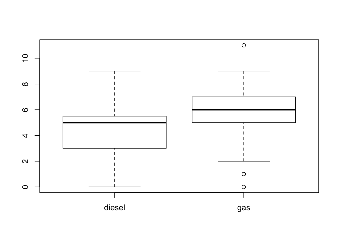
FIGURE 11.1: Box Plots of Differences in MPG

We conduct inference for each fuel type separately. However, since the sample size for cars that run on diesel is only 20, one may have concerns regarding the application of methods that assume a large sample size to a sample size this small.

11.3.1 Confidence Intervals for a Normal Mean

Consider the construction of a confidence interval for the expectation of a Normal measurement. In the previous section, when dealing with the construction of a confidence interval for the expectation, we exploited the Central Limit Theorem in order to identify that the distribution of the standardized sample average \((\bar X - \Expec(X))/\sqrt{\Var(X)/n}\) is, approximately, standard Normal. Afterwards, we substituted the standard deviation of the measurement by the sample standard deviation \(S\), which was an accurate estimator of the former due to the magnitude sample size.

In the case where the measurements themselves are Normally distributed one can identify the exact distribution of the standardized sample average, with the sample variance substituting the variance of the measurement: \((\bar X - \Expec(X))/(S/\sqrt{n})\). This specific distribution is called the Student’s \(t\)-distribution, or simply the \(t\)-distribution.

The \(t\)-distribution is bell shaped and symmetric. Overall, it looks like the standard Normal distribution but it has wider tails. The \(t\)-distribution is characterized by a parameter called the number of degrees of freedom. In the current setting, where we deal with the standardized sample average (with the sample variance substituting the variance of the measurement) the number of degrees of freedom equals the number of observations associated with the estimation of the variance, minus 1. Hence, if the sample size is \(n\) and if the measurement is Normally distributed then the standardized sample average (with \(S\) substituting the standard deviation of the measurement) has a \(t\)-distribution on \((n-1)\) degrees of freedom. We use \(t_{(n-1)}\) to denote this \(t\)-distribution.

The R system contains functions for the computation of the density, the cumulative probability function and the percentiles of the \(t\)-distribution, as well as for the simulation of a random sample from this distribution. Specifically, the function “qt” computes the percentiles of the \(t\)-distribution. The first argument to the function is a probability and the second argument is the number of degrees of freedom. The output of the function is the percentile associated with the probability of the first argument. Namely, it is a value such that the probability that the \(t\)-distribution is below the value is equal to the probability in the first argument.

For example, let “n” be the sample size. The output of the expression “qt(0.975,n-1)” is the 0.975-percentile of the \(t\)-distribution on \((n-1)\) degrees of freedom. By definition, 97.5% of the \(t\)-distribution are below this value and 2.5% are above it. The symmetry of the \(t\) distribution implies that 2.5% of the distribution is below the negative of this value. The middle part of the distribution is bracketed by these two values: \([-\mbox{\texttt{qt(0.975,n-1)}}, \mbox{\texttt{qt(0.975,n-1)}}]\), and it contains 95% of the distribution.

Summarizing the above claims in a single formula produces the statement:

\[\frac{\bar X - \Expec(X)}{S/\sqrt{n}} \sim t_{(n-1)} \quad \Longrightarrow \quad \Prob \bigg(\bigg|\frac{\bar X - \Expec(X)}{S/\sqrt{n}}\bigg| \leq \mbox{\texttt{qt(0.975,n-1)}} \bigg) = 0.95\;.\] Notice that the equation associated with the probability is not an approximation but an exact relation⁴⁸. Rewriting the event that is described in the probability in the form of a confidence interval, produces

\[\bar X \pm \mbox{\texttt{qt(0.975,n-1)}}\cdot S/ \sqrt{n}\] as a confidence interval for the expectation of the Normal measurement with a confidence level of 95%.

The structure of the confidence interval for the expectation of a Normal measurement is essentially identical to the structure proposed in the previous section. The only difference is that the number 1.96, the percentile of the standard Normal distribution, is substituted by the percentile of the \(t\)-distribution.

Consider the construction of a confidence interval for the expected difference in fuel consumption between highway and urban driving conditions. In order to save writing we created two new variables; a factor called “fuel” that contains the data on the fuel type of each car, and a numerical vector called “dif.mpg” that contains the difference between highway and city fuel consumption for each car type:

fuel <- cars$fuel.type
dif.mpg <- cars$highway.mpg - cars$city.mpg

We are interested in confidence intervals based on the data stored in the variable “dif.mpg”. One confidence interval will be associated with the level “diesel” of the factor “fuel” and the other will be associated with the level “gas” of the same factor.

In order to compute these confidence intervals we need to compute, for each level of the factor “fuel”, the sample average and the sample standard deviation of the data points of the variable “dif.mpg” that are associated with that level.

It is convenient to use the function “tapply” for this task. This function uses three arguments. The first argument is the sequence of values over which we want to carry out some computation. The second argument is a factor. The third argument is a name of a function that is used for the computation. The function “tapply” applies the function in the third argument to each sub-collection of values of the first argument. The sub-collections are determined by the levels of the second argument.

Sounds complex but it is straightforward enough to apply:

tapply(dif.mpg,fuel,mean)

##   diesel      gas 
## 4.450000 5.648649

tapply(dif.mpg,fuel,sd)

##   diesel      gas 
## 2.781045 1.433607

Sample averages are computed in the first application of the function “tapply”. Observe that an average was computed for cars that run on diesel and an average was computed for cars that run on gas. In both cases the average corresponds to the difference in fuel consumption. Similarly, the standard deviations were computed in the second application of the function. We obtain that the point estimates of the expectation for diesel and gas cars are 4.45 and 5.648649, respectively and the point estimates for the standard deviation of the variable are 2.781045 and 1.433607.

Let us compute the confidence interval for each type of fuel:

x.bar <- tapply(dif.mpg,fuel,mean)
s <- tapply(dif.mpg,fuel,sd)
n <- c(20,185)
x.bar - qt(0.975,n-1)*s/sqrt(n)

##   diesel      gas 
## 3.148431 5.440699

x.bar + qt(0.975,n-1)*s/sqrt(n)

##   diesel      gas 
## 5.751569 5.856598

The objects “x.bar” and “s” contain the sample averages and sample standard deviations, respectively. Both are sequences of length two, with the first component referring to “diesel” and the second component referring to “gas”. The object “n” contains the two sample sizes, 20 for “diesel” and 185 for “gas”. In the expression next to last the lower boundary for each of the confidence intervals is computed and in the last expression the upper boundary is computed. The confidence interval for the expected difference in diesel cars is \([3.148431, 5.751569]\). and the confidence interval for cars using gas is \([5.440699, 5.856598]\).

The 0.975-percentiles of the \(t\)-distributions are computed with the expressions “qt(0.025,n-1)”:

qt(0.975,n-1)

## [1] 2.093024 1.972941

The second argument of the function “qt” is a sequence with two components, the number 19 and the number 184. Accordingly, The first position in the output of the function is the percentile associated with 19 degrees of freedom and the second position is the percentile associated to 184 degrees of freedom.

Compare the resulting percentiles to the 0.975-percentile of the standard Normal distribution, which is essentially equal to 1.96. When the sample size is small, 20 for example, the percentile of the \(t\)-distribution is noticeably larger than the percentile of the standard Normal. However, for a larger sample size the percentiles, more or less, coincide. It follows that for a large sample the method proposed in Subsection 11.2.2 and the method discussed in this subsection produce essentially the same confidence intervals.

11.3.2 Confidence Intervals for a Normal Variance

The next task is to compute confidence intervals for the variance of a Normal measurement. The main idea in the construction of a confidence interval is to identify the distribution of a random variable associated with the parameter of interest. A region that contains 95% of the distribution of the random variable (or, more generally, the central part of the distribution of probability equal to the confidence level) is identified. The confidence interval results from the reformulation of the event associated with that region. The new formulation puts the parameter between a lower limit and an upper limit. These lower and the upper limits are computed from the data and they form the boundaries of the confidence interval.

We start with the sample variance, \(S^2 = \sum_{i=1}^n (X_i - \bar X)^2/(n-1)\), which serves as a point estimator of the parameter of interest. When the measurements are Normally distributed then the random variable \((n-1)S^2/\sigma^2\) possesses a special distribution called the chi-square distribution. (Chi is the Greek letter \(\chi\), which is read “Kai”.) This distribution is associated with the sum of squares of Normal variables. It is parameterized, just like the \(t\)-distribution, by a parameter called the number of degrees of freedom. This number is equal to \((n-1)\) in the situation we discuss. The chi-square distribution on \((n-1)\) degrees of freedom is denoted with the symbol \(\chi^2_{(n-1)}\).

The R system contains functions for the computation of the density, the cumulative probability function and the percentiles of the chi-square distribution, as well as for the simulation of a random sample from this distribution. Specifically, the percentiles of the chi-square distribution are computed with the aid of the function “qchisq”. The first argument to the function is a probability and the second argument is the number of degrees of freedom. The output of the function is the percentile associated with the probability of the first argument. Namely, it is a value such that the probability that the chi-square distribution is below the value is equal to the probability in the first argument.

For example, let “n” be the sample size. The output of the expression “qt(0.975,n-1)” is the 0.975-percentile of the chi-square distribution. By definition, 97.5% of the chi-square distribution are below this value and 2.5% are above it. Similarly, the expression “qchisq(0.025,n-1)” is the 0.025-percentile of the chi-square distribution, with 2.5% of the distribution below this value. Notice that between these two percentiles, namely within the interval \([\mbox{\texttt{qchisq(0.025,n-1)}}, \mbox{\texttt{qchisq(0.975,n-1)}}]\), are 95% of the chi-square distribution.

We may summarize that for Normal measurements:

\[\begin{aligned} \lefteqn{(n-1)S^2/\sigma^2 \sim \chi^2_{(n-1)} \quad \Longrightarrow }\\ & \Prob \big( \mbox{\texttt{qchisq(0.025,n-1)}} \leq (n-1)S^2/\sigma^2 \leq \mbox{\texttt{qchisq(0.975,n-1)}} \big) = 0.95\;.\end{aligned}\] The chi-square distribution is not symmetric. Therefore, in order to identify the region that contains 95% of the distribution region we have to compute both the 0.025- and the 0.975-percentiles of the distribution.

The event associated with the 95% region is rewritten in a form that puts the parameter \(\sigma^2\) in the center:

\[\big\{(n-1)S^2/\mbox{\texttt{qchisq(0.975,n-1)}} \leq \sigma^2 \leq (n-1)S^2/\mbox{\texttt{qchisq(0.025,n-1)}}\big\}\;.\] The left most and the right most expressions in this event mark the end points of the confidence interval. The structure of the confidence interval is:

\[\big[\{(n-1)/\mbox{\texttt{qchisq(0.975,n-1)}}\}\times S^2,\;\{(n-1)/\mbox{\texttt{qchisq(0.025,n-1)}}\}\times S^2\big]\;.\] Consequently, the confidence interval is obtained by the multiplication of the estimator of the variance by a ratio between the number of degrees of freedom (\(n-1\)) and an appropriate percentile of the chi-square distribution. The percentile on the left hand side is associated with the larger probability (making the ratio smaller) and the percentile on the right hand side is associated with the smaller probability (making the ratio larger).

Consider, specifically, the confidence intervals for the variance of the measurement “diff.mpg” for cars that run on diesel and for cars that run on gas. Here, the size of the samples is 20 and 185, respectively:

(n-1)/qchisq(0.975,n-1)

## [1] 0.5783456 0.8234295

(n-1)/qchisq(0.025,n-1)

## [1] 2.133270 1.240478

The ratios that are used in the left hand side of the intervals are 0.5783456 and 0.8234295, respectively. Both ratios are less than one. On the other hand, the ratios associated with the other end of the intervals, 2.133270 and 1.240478, are both larger than one.

Let us compute the point estimates of the variance and the associated confidence intervals. Recall that the object “s” contains the sample standard deviations of the difference in fuel consumption for diesel and for gas cars. The object “n” contains the two sample sizes:

s^2

##   diesel      gas 
## 7.734211 2.055229

(n-1)*s^2/qchisq(0.975,n-1)

##   diesel      gas 
## 4.473047 1.692336

(n-1)*s^2/qchisq(0.025,n-1)

##    diesel       gas 
## 16.499155  2.549466

The variance of the difference in fuel consumption for diesel cars is estimated to be 7.734211 with a 95%-confidence interval of \([4.473047, 16.499155]\) and for cars that use gas the estimated variance is 2.055229, with a confidence interval of \([1.692336, 2.549466]\).

As a final example in this section let us simulate the confidence level for a confidence interval for the expectation and for a confidence interval for the variance of a Normal measurement. In this simulation we assume that the expectation is equal to \(\mu = 3\) and the variance is equal to \(\sigma^2 = 3^2 = 9\). The sample size is taken to be \(n=20\). We start by producing the sampling distribution of the sample average \(\bar X\) and of the sample standard deviation \(S\):

mu <- 4
sig <- 3
n <- 20
X.bar <- rep(0,10^5)
S <- rep(0,10^5)
for(i in 1:10^5) {
  X <- rnorm(n,mu,sig)
  X.bar[i] <- mean(X)
  S[i] <- sd(X)
}

Consider first the confidence interval for the expectation:

mu.LCL <- X.bar - qt(0.975,n-1)*S/sqrt(n)
mu.UCL <- X.bar + qt(0.975,n-1)*S/sqrt(n)
mean((mu >= mu.LCL) & (mu <= mu.UCL))

## [1] 0.95009

The nominal significance level of the confidence interval is 95%, which is practically identical to the confidence level that was computed in the simulation.

The confidence interval for the variance is obtained in a similar way. The only difference is that we apply now different formulae for the computation of the upper and lower confidence limits:

var.LCL <- (n-1)*S^2/qchisq(0.975,n-1)
var.UCL <- (n-1)*S^2/qchisq(0.025,n-1)
mean((sig^2 >= var.LCL) & (sig^2 <= var.UCL))

## [1] 0.94959

Again, we obtain that the nominal confidence level of 95% coincides with the confidence level computed in the simulation.

11.4 Choosing the Sample Size

One of the more important contributions of Statistics to research is providing guidelines for the design of experiments and surveys. A well planed experiment may produce accurate enough answers to the research questions while optimizing the use of resources. On the other hand, poorly planed trials may fail to produce such answers or may waste valuable resources.

Unfortunately, in this book we do not cover the subject of experiment design. Still, we would like to give a brief discussion of a narrow aspect in design: The selection of the sample size.

An important consideration at the stage of the planning of an experiment or a survey is the number of observations that should be collected. Indeed, having a larger sample size is usually preferable from the statistical point of view. However, an increase in the sample size typically involves an increase in expenses. Thereby, one would prefer to collect the minimal number of observations that is still sufficient in order to reach a valid conclusion.

As an example, consider an opinion poll aimed at the estimation of the proportion in the population of those that support a specific candidate that considers running for an office. How large the sample must be in order to assure, with high probability, that the percentage in the sample of supporters is within 0.5% of the percentage in the population? Within 0.25%?

A natural way to address this problem is via a confidence interval for the proportion. If the range of the confidence interval is no more than 0.05 (or 0.025 in the other case) then with a probability equal to the confidence level it is assured that the population relative frequency is within the given distance from the sample proportion.

Consider a confidence level of 95%. Recall that the structure of the confidence interval for the proportion is \(\hat P \pm 1.96 \cdot \{\hat P (1-\hat P)/n\}^{1/2}\). The range of the confidence interval is \(1.96 \cdot \{\hat P (1-\hat P)/n\}^{1/2}\). How large should \(n\) be in order to guarantee that the range is no more than 0.05?

The answer to this question depends on the magnitude of \(\hat P (1-\hat P)\), which is a random quantity. Luckily, one may observe that the maximal value⁴⁹ of the quadratic function \(f(p) = p (1-p)\) is 1/4. It follows that

\[1.96 \cdot \{\hat P (1-\hat P)/n\}^{1/2} \leq 1.96 \cdot \{0.25/n\}^{1/2} = 0.98/\sqrt{n}\;.\] Finally,

\[0.98/\sqrt{n} \leq 0.05 \quad \Longrightarrow \quad \sqrt{n} \geq 0.98/0.05 = 19.6 \quad \Longrightarrow \quad n \geq (19.6)^2 = 384.16\;.\] The conclusion is that \(n\) should be larger than 384 in order to assure the given range. For example, \(n=385\) should be sufficient.

If the request is for an interval of range 0.025 then the last line of reasoning should be modified accordingly:

\[0.98/\sqrt{n} \leq 0.025 \quad \Longrightarrow \quad \sqrt{n} \geq \frac{0.98}{0.025} = 39.2 \quad \Longrightarrow \quad n \geq (39.2)^2 = 1536.64\;.\] Consequently, \(n=1537\) will do. Increasing the accuracy by 50% requires a sample size that is 4 times larger.

More examples that involve selection of the sample size will be considered as part of the homework.

11.5 Exercises

Exercise 11.1 This exercise deals with an experiment that was conducted among students. The aim of the experiment was to assess the effect of rumors and prior reputation of the instructor on the evaluation of the instructor by her students. The experiment was conducted by Towler and Dipboye⁵⁰. This case study is taken from the Rice Virtual Lab in Statistics. More details on this case study can be found in the case study “Instructor Reputation and Teacher Ratings” that is presented in that site.

The experiment involved 49 students that were randomly assigned to one of two conditions. Before viewing the lecture, students were give one of two “summaries” of the instructor’s prior teaching evaluations. The first type of summary, i.e. the first condition, described the lecturer as a charismatic instructor. The second type of summary (second condition) described the lecturer as a punitive instructor. We code the first condition as “C” and the second condition as “P”. All subjects watched the same twenty-minute lecture given by the exact same lecturer. Following the lecture, subjects rated the lecturer.

The outcomes are stored in the file “teacher.csv”. The file can be found on the internet at http://pluto.huji.ac.il/~msby/StatThink/Datasets/teacher.csv. Download this file to your computer and store it in the working directory of R. Read the content of the file into an R data frame. Produce a summary of the content of the data frame and answer the following questions:

1. Identify, for each variable in the file “teacher.csv”, the name and the type of the variable (factor or numeric).

2. Estimate the expectation and the standard deviation among all students of the rating of the teacher.

3. Estimate the expectation and the standard deviation of the rating only for students who were given a summary that describes the teacher as charismatic.

4. Construct a confidence interval of 99% confidence level for the expectation of the rating among students who were given a summary that describes the teacher as charismatic. (Assume the ratings have a Normal distribution.)

5. Construct a confidence interval of 90% confidence level for the variance of the rating among students who were given a summary that describes the teacher as charismatic. (Assume the ratings have a Normal distribution.)

Exercise 11.2 Twenty observations are used in order to construct a confidence interval for the expectation. In one case, the construction is based on the Normal approximation of the sample average and in the other case it is constructed under the assumption that the observations are Normally distributed. Assume that in reality the measurement is distributed \(\mathrm{Exponential}(1/4)\).

1. Compute, via simulation, the actual confidence level for the first case of a confidence interval with a nominal confidence level of 95%.

2. Compute, via simulation, the actual confidence level for the second case of a confidence interval with a nominal confidence level of 95%.

3. Which of the two approaches would you prefer?

Exercise 11.3 Insurance companies are interested in knowing the population percent of drivers who always buckle up before riding in a car.

1. When designing a study to determine this proportion, what is the minimal sample size that is required for a 99% confident that the population proportion is accurately estimated, up to an error of 0.03?

2. Suppose that the insurance companies did conduct the study by surveying 400 drivers. They found that 320 of the drives claim to always buckle up. Produce an 80% confidence interval for the population proportion of drivers who claim to always buckle up.

11.6 Summary

Glossary

Confidence Interval:

An interval that is most likely to contain the population parameter.

Confidence Level:

The sampling probability that random confidence intervals contain the parameter value. The confidence level of an observed interval indicates that it was constructed using a formula that produces, when applied to random samples, such random intervals.

t-Distribution:

A bell-shaped distribution that resembles the standard Normal distribution but has wider tails. The distribution is characterized by a positive parameter called degrees of freedom.

Chi-Square Distribution:

A distribution associated with the sum of squares of Normal random variable. The distribution obtains only positive values and it is not symmetric. The distribution is characterized by a positive parameter called degrees of freedom.

Discuss in the forum

When large samples are at hand one may make fewer a-priori assumptions regarding the exact form of the distribution of the measurement. General limit theorems, such as the Central Limit Theorem, may be used in order to establish the validity of the inference under general conditions. On the other hand, for small sample sizes one must make strong assumptions with respect to the distribution of the observations in order to justify the validity of the procedure.

It may be claimed that making statistical inferences when the sample size is small is worthless. How can one trust conclusions that depend on assumptions regarding the distribution of the observations, assumptions that cannot be verified? What is your opinion?

For illustration consider the construction of a confidence interval. Confidence interval for the expectation is implemented with a specific formula. The significance level of the interval is provable when the sample size is large or when the sample size is small but the observations have a Normal distribution. If the sample size is small and the observations have a distribution different from the Normal then the nominal significance level may not coincide with the actual significance level.

Formulas for Confidence Intervals, 95% Confidence Level:

• Expectation: \(\bar x \pm \mbox{\texttt{qnorm(0.975)}} \cdot s/\sqrt{n}\).

• Probability: \(\bar p \pm \mbox{\texttt{qnorm(0.975)}} \cdot \hat p(1-\hat p)/\sqrt{n}\).

• Normal Expectation: \(\bar x \pm \mbox{\texttt{qt(0.975,n-1)}} \cdot s/\sqrt{n}\).

• Normal Expectation: \(\big[\frac{n-1}{\mbox{\texttt{qchisq(0.975,n-1)}}} s^2 ,\;\frac{n-1}{\mbox{\texttt{qchisq(0.025,n-1)}}} s^2\big]\).

---

46. Observe that \(|\bar X - \Expec(X)| = |\Expec(X) -\bar X |\) and therefore \(\big\{|\bar X - \Expec(X)| \leq 1.96 \cdot \sqrt{\Var(X)/n} \big\} =\big\{| \Expec(X)-\bar X | \leq 1.96 \cdot \sqrt{\Var(X)/n} \big\}\). From the definition of the absolute value we obtain that the last expression is equal to \(\big\{-1.96 \cdot \sqrt{\Var(X)/n} \leq \Expec(X)-\bar X \leq 1.96 \cdot \sqrt{\Var(X)/n} \big\}\). Moving the average to the other side of the inequality (for both inequalities involved) produces the representation \(\big\{\bar X-1.96 \cdot \sqrt{\Var(X)/n} \leq \Expec(X)\leq \bar X + 1.96 \cdot \sqrt{\Var(X)/n} \big\}\).↩

47. The sample variance, that serves as the estimator of the variance, is computed from the sample using the formula: \(S^2 = \sum_{i=1}^n (X_i-\bar X)^2/(n-1)\).↩

48. When the measurement is Normally distributed.↩

49. The derivative is \(f'(p) = 1-2p\). Solving \(f'(p)=0\) produces \(p=1/2\) as the maximizer. Plugging this value in the function gives \(1/4\) as the maximal value of the function.↩

50. Towler, A. and Dipboye, R. L. (1998). The effect of instructor reputation and need for cognition on student behavior (poster presented at American Psychological Society conference, May 1998).↩