Chapter 2 Sampling and Data Structures

2.1 Student Learning Objectives

In this chapter we deal with issues associated with the data that is obtained from a sample. The variability associated with this data is emphasized and critical thinking about validity of the data encouraged. A method for the introduction of data from an external source into R is proposed and the data types used by R for storage are described. By the end of this chapter, the student should be able to:

Recognize potential difficulties with sampled data.
Import data into R.
Organize your work in R-scripts.
Create and interpret frequency tables.

2.2 The Sampled Data

The aim in statistics is to learn the characteristics of a population on the basis of a sample selected from the population. An essential part of this analysis involves consideration of variation in the data.

2.2.1 Variation in Data

Variation is given a central role in statistics. To some extent the assessment of variation and the quantification of its contribution to uncertainties in making inference is the statistician’s main concern.

Variation is present in any set of data. For example, 16-ounce cans of beverage may contain more or less than 16 ounces of liquid. In one study, eight 16 ounce cans were measured and produced the following amount (in ounces) of beverage:

\[15.8,16.1,15.2,14.8,15.8,15.9,16.0,15.5\] Measurements of the amount of beverage in a 16-ounce may vary because the conditions of measurement varied or because the exact amount, 16 ounces of liquid, was not put into the cans. Manufacturers regularly run tests to determine if the amount of beverage in a 16-ounce can falls within the desired range.

2.2.2 Variation in Samples

Two random samples from the same population, while resembling the population, will nonetheless be different from each other. Suppose Doreen and Jung both decide to study the average amount of time students sleep each night and use all students at their college as the population. Doreen may decide to sample randomly 50 students from the entire body of collage students. Jung also collects a random sample of 50 students. The randomness in the sampling will result in Doreen’s sample consisting in different students than Jung’s sample and therefore exhibit different variation in sleeping patterns purely arising from sampling variation (as oppossed to variation arising from error in measuring sleep for a given students).

Both samples will however resemble the population. If Doreen and Jung took larger samples (i.e. the number of data values is increased), their samples and their characteristics, for example the average amount of time a student sleeps, would be closer to the actual population value. But still, their samples would still be, most probably, different from each other.

The size of a sample (often called the number of observations) plays a key role in determining the uncertainty regarding what we can learn from our data about the population. The examples you have seen in this book so far have been small for convenience, but are usually too small to learn something with relative certainty about a population. Samples of only a few hundred observations, or even smaller, can however be sufficient. In polling, samples that are from 1200 to 1500 observations are considered large enough and good enough if the survey is random and is well done. The theory of statistical inference, that is the subject matter of the second part of this book, provides justification for these claims as well as techniques to quantify the uncertainty arising from random sampling and make decisions about sample sizes.

Finally, for the reasons outlined above, if an investigator collects data they will often vary somewhat from the data someone else is taking for the same purpose. However, if two investigators or more, are taking data from the same source and get very different results, it is time for them to reevaluate their data-collection methods and data recording accuracy.

2.2.3 Frequency

The primary way of summarizing the variability of data is via the frequency distribution. Consider an example. Twenty students were asked how many hours they worked per day. Their responses, in hours, are listed below:

\[5,\; 6,\; 3,\; 3,\; 2,\; 4,\; 7,\; 5,\; 2,\; 3,\; 5,\; 6,\; 5,\; 4,\; 4,\; 3,\; 5,\; 2,\; 5,\; 3\] Let us create an R object by the name “work.hours” that contains these data:

work.hours <- c(5,6,3,3,2,4,7,5,2,3,5,6,5,4,4,3,5,2,5,3)

Next, let us create a table that summarizes the different values of working hours and the frequency in which these values appear in the data:

table(work.hours)

## work.hours
## 2 3 4 5 6 7 
## 3 5 3 6 2 1

Recall that the function “table” takes as input a sequence of data and produces as output the frequencies of the different values.

We may have a clearer understanding of the meaning of the output of the function “table” if we presented outcome as a frequency listing the different data values in ascending order and their frequencies. For that end we may apply the function “data.frame” to the output of the “table” function and obtain:

data.frame(table(work.hours))

##   work.hours Freq
## 1          2    3
## 2          3    5
## 3          4    3
## 4          5    6
## 5          6    2
## 6          7    1

A frequency is the number of times a given datum occurs in a data set. According to the table above, there are three students who work 2 hours, five students who work 3 hours, etc. The total of the frequency column, 20, represents the total number of students included in the sample.

The function “data.frame” transforms its input into a data frame, which is the standard way of storing statistical data. We will introduce data frames in more detail in Section 2.3 below.

A relative frequency is the fraction of times a value occurs. To find the relative frequencies, divide each frequency by the total number of students in the sample – 20 in this case. Relative frequencies can be written as fractions, percents, or decimals.

As an illustration let us compute the relative frequencies in our data:

freq <- table(work.hours)
freq

## work.hours
## 2 3 4 5 6 7 
## 3 5 3 6 2 1

sum(freq)

## [1] 20

freq/sum(freq)

## work.hours
##    2    3    4    5    6    7 
## 0.15 0.25 0.15 0.30 0.10 0.05

We stored the frequencies in an object called “freq”. The content of the object are the frequencies 3, 5, 3, 6, 2 and 1. The function “sum” sums the components of its input. The sum of the frequencies is the sample size , the total number of students that responded to the survey, which is 20. Hence, when we apply the function “sum” to the object “freq” we get 20 as an output.

The outcome of dividing an object by a number is a division of each element in the object by the given number. Therefore, when we divide “freq” by “sum(freq)” (the number 20) we get a sequence of relative frequencies. The first entry to this sequence is \(3/20 = 0.15\), the second entry is \(5/20 = 0.25\), and the last entry is \(1/20 = 0.05\). The sum of the relative frequencies should always be equal to 1:

sum(freq/sum(freq))

## [1] 1

The cumulative relative frequency is the accumulation of previous relative frequencies. To find the cumulative relative frequencies, add all the previous relative frequencies to the relative frequency of the current value. Alternatively, we may apply the function “cumsum” to the sequence of relative frequencies:

cumsum(freq/sum(freq))

##    2    3    4    5    6    7 
## 0.15 0.40 0.55 0.85 0.95 1.00

Observe that the cumulative relative frequency of the smallest value 2 is the frequency of that value (0.15). The cumulative relative frequency of the second value 3 is the sum of the relative frequency of the smaller value (0.15) and the relative frequency of the current value (0.25), which produces a total of \(0.15 + 0.25 = 0.40\). Likewise, for the third value 4 we get a cumulative relative frequency of \(0.15 + 0.25 + 0.15 = 0.55\). The last entry of the cumulative relative frequency column is one, indicating that one hundred percent of the data has been accumulated.

The computation of the cumulative relative frequency was carried out with the aid of the function “cumsum”. This function takes as an input argument a numerical sequence and produces as output a numerical sequence of the same length with the cumulative sums of the components of the input sequence.

2.2.4 Critical Evaluation

Inappropriate methods of sampling and data collection may produce samples that do not represent the target population. A naïve application of statistical analysis to such data may produce misleading conclusions.

Consequently, it is important to evaluate critically the statistical analyses we encounter before accepting the conclusions that are obtained as a result of these analyses. Common problems that occurs in data that one should be aware of include:

Problems with Samples:: A sample should be representative of the population. A sample that is not representative of the population is biased. Biased samples may produce results that are inaccurate and not valid.
Data Quality:: Avoidable errors may be introduced to the data via inaccurate handling of forms, mistakes in the input of data, etc. Data should be cleaned from such errors as much as possible.
Self-Selected Samples:: Responses only by people who choose to respond, such as call-in surveys, that are often biased.
Sample Size Issues:: Samples that are too small may be unreliable. Larger samples, when possible, are better. In some situations, small samples are unavoidable and can still be used to draw conclusions. Examples: Crash testing cars, medical testing for rare conditions.
Undue Influence:: Collecting data or asking questions in a way that influences the response.
Causality:: A relationship between two variables does not mean that one causes the other to occur. They may both be related (correlated) because of their relationship to a third variable.
Self-Funded or Self-Interest Studies:: A study performed by a person or organization in order to support their claim. Is the study impartial? Read the study carefully to evaluate the work. Do not automatically assume that the study is good but do not automatically assume the study is bad either. Evaluate it on its merits and the work done.
Misleading Use of Data:: Improperly displayed graphs and incomplete data.
Confounding:: Confounding in this context means confusing. When the effects of multiple factors on a response cannot be separated. Confounding makes it difficult or impossible to draw valid conclusions about the effect of each factor.

2.3 Reading External Data into `R`

In the examples so far the size of the data set was very small and we were able to input the data directly into R with the use of the function “c”. In more practical settings the data sets to be analyzed are much larger and it is very inefficient to enter them manually. In this section we learn how to read data from a file in the Comma Separated Values (CSV) format.

The file “ex1.csv” contains data on the sex and height of 100 individuals. This file is given in the CSV format. The file can be found on the internet at http://pluto.huji.ac.il/~msby/StatThink/Datasets/ex1.csv. We will discuss the process of reading data from a file into R and use this file as an illustration.

2.3.1 Saving the File and Setting the Working Directory

Before the file is read into R you should obtain a copy of the file and store it in some directory on the computer and read the file from that directory. We recommend that you create a special directory in which you keep all the material associated with this course. In the explanations provided below we assume that the directory to which the file is stored in called “IntroStat”.

Files in the CSV format are ordinary text files. They can be created manually or as a result of converting data stored in a different format into this particular format. A common way to produce, browse and edit CSV files is by the use of a standard electronic spreadsheet programs such as Excel or Calc. The Excel spreadsheet is part of the Microsoft’s Office suite. The Calc spreadsheet is part of the free LibreOffice suite. Note however that you should never edit raw data files directly. Keep them in a separate directory and never overwrite them with changes. Any changes you make to the data should be retraceable and documented through R-scripts and the changed data should be saved under a different name.

Opening a CSV file by a spreadsheet program displays a spreadsheet with the content of the file. Values in the cells of the spreadsheet may be modified directly. (However, when saving, one should pay attention to save the file in the CVS format.) Similarly, new CSV files may be created by the entering of the data in an empty spreadsheet. The first row should include the name of the variable, preferably as a single character string with no empty spaces. The following rows may contain the data values associated with this variable. When saving, the spreadsheet should be saved in the CSV format by the use of the “" dialog and choosing there the option of CSV in the “Save by Type” selection.

After saving a file with the data in a directory, R should be notified where the file is located in order to be able to read it. A simple way of doing so is by setting the directory with the file as R’s working directory. The working directory is the first place R is searching for files. Files produced by R are saved in that directory. In RStudio one may set the working directory of the active R session to be some target directory in the “Files” panel The dialog is opened by clicking on “More” on the left hand side of the toolbar on the top of the Files panel. In the menu that opens selecting the option of “Set As Working Directory” will start the dialog. (See Figure 2.1.) Browsing via this dialog window to the directory of choice, selecting it, and approving the selection by clicking the “OK” bottom in the dialog window will set the directory of choice as the working directory of R.

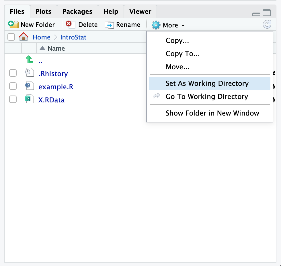
FIGURE 2.1: Changing The Working Directory

A full statistical ananlysis will typically involve a non-negligible number of steps. Retracing these steps in retrospect is often difficult without proper documentation. So while working from the R-console is a good way to develop (steps) in an analysis, you will need a way to document your work in order for your the analysis to be reproducible. Rather than to work only from the R-console (and change the working directory every time that R is opened manually), it is better to organize your R-code in so-called scripts. R-scripts are plain text files which contain the R-commands that perform your analysis. Executing these scripts will perform your full analysis and thereby make your work reproducible.

Figure 2.2 shows how to create an R-script in RStudio. This is done by clicking on the first button on the main toolbar in RStudio. This will popup a menu where you can click on R-script. RStudio will then create a new empty R-script in the editing panel as shown in Figure 2.3. Here you can add the R-commands that will perform your analysis. Make sure to save your new script. Finally note that you can select one or several lines in your R-script and click on the `Run’ button in the toolbar to execute them in the R-console.

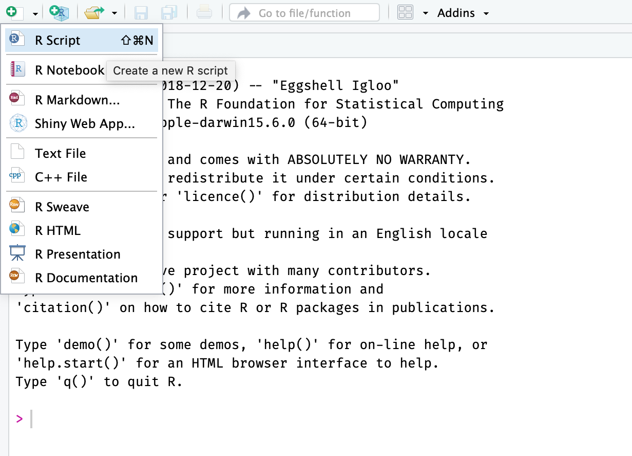
FIGURE 2.2: Creating an R-script

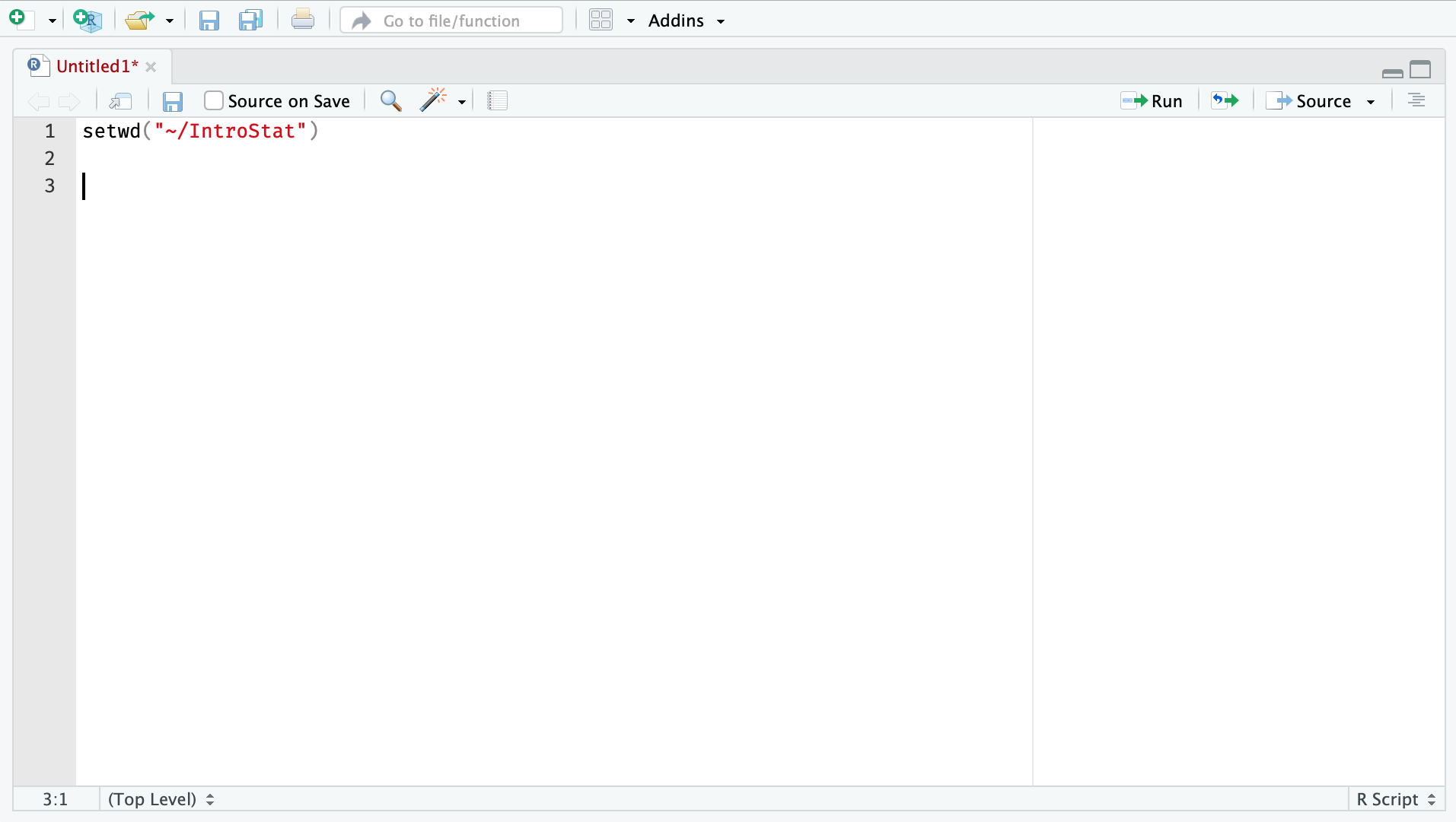
FIGURE 2.3: Editing an R-script

In the rest of this book we assume that a designated directory is set as R’s working directory and that all external files that need to be read into R, such as “ex1.csv” for example, are saved in that working directory. Once a working directory has been set then the history of subsequent R sessions is stored in that directory. Hence, if you choose to save the image of the session when you end the session then objects created in the session will be uploaded the next time the R Console is opened.

2.3.2 Reading a CSV File into `R`

Now that a copy of the file “ex1.csv” is placed in the working directory we would like to read its content into R. Reading of files in the CSV format can be carried out with the R function “read.csv”. To read the file of the example we run the following line of code in the R Console panel:

ex.1 <- read.csv("_data/ex1.csv")

The function “read.csv” takes as an input argument the address of a CSV file and produces as output a data frame object with the content of the file. Notice that the address is placed between double-quotes. If the file is located in the working directory then giving the name of the file as an address is sufficient².

Consider the content of that R object “ex.1” that was created by the previous expression, by inspecting the first part using the function “head()”:

head(ex.1)

##        id    sex height
## 1 5696379 FEMALE    182
## 2 3019088   MALE    168
## 3 2038883   MALE    172
## 4 1920587 FEMALE    154
## 5 6006813   MALE    174
## 6 4055945 FEMALE    176

The object “ex.1”, the output of the function “read.csv” is a data frame. Data frames are the standard tabular format of storing statistical data. The columns of the table are called variables and correspond to measurements. In this example the three variables are:

id:: A 7 digits number that serves as a unique identifier of the subject.
sex:: The sex of each subject. The values are either “MALE” or “FEMALE”.
height:: The height (in centimeter) of each subject. A numerical value.

When the values of the variable are numerical we say that it is a quantitative variable or a numeric variable. On the other hand, if the variable has qualitative or level values we say that it is a factor. In the given example, sex is a factor and height is a numeric variable.

The rows of the table are called observations and correspond to the subjects. In this data set there are 100 subjects, with subject number 1, for example, being a female of height 182 cm and identifying number 5696379. Subject number 98, on the other hand, is a male of height 195 cm and identifying number 9383288.

2.3.3 Data Types

The columns of R data frames represent variables, i.e. measurements recorded for each of the subjects in the sample. R associates with each variable a type that characterizes the content of the variable. The two major types are

Factors, or Qualitative Data. The type is “factor”.
Quantitative Data. The type is “numeric”.

Factors are the result of categorizing or describing attributes of a population. Hair color, blood type, ethnic group, the car a person drives, and the street a person lives on are examples of qualitative data. Qualitative data are generally described by words or letters. For instance, hair color might be black, dark brown, light brown, blonde, gray, or red. Blood type might be AB+, O-, or B+. Qualitative data are not as widely used as quantitative data because many numerical techniques do not apply to the qualitative data. For example, it does not make sense to find an average hair color or blood type.

Quantitative data are always numbers and are usually the data of choice because there are many methods available for analyzing such data. Quantitative data are the result of counting or measuring attributes of a population. Amount of money, pulse rate, weight, number of people living in your town, and the number of students who take statistics are examples of quantitative data.

Quantitative data may be either discrete or continuous. All data that are the result of counting are called quantitative discrete data. These data take on only certain numerical values. If you count the number of phone calls you receive for each day of the week, you may get results such as 0, 1, 2, 3, etc. On the other hand, data that are the result of measuring on a continuous scale are quantitative continuous data, assuming that we can measure accurately. Measuring angles in radians may result in the numbers \(\frac{\pi}{6}\), \(\frac{\pi}{3}\), \(\frac{\pi}{2}\), \(\pi\), \(\frac{3\pi}{4}\), etc. If you and your friends carry backpacks with books in them to school, the numbers of books in the backpacks are discrete data and the weights of the backpacks are continuous data.

The data are the number of books students carry in their backpacks. You sample five students. Two students carry 3 books, one student carries 4 books, one student carries 2 books, and one student carries 1 book. The numbers of books (3, 4, 2, and 1) are the quantitative discrete data.

The data are the weights of the backpacks with the books in it. You sample the same five students. The weights (in pounds) of their backpacks are 6.2, 7, 6.8, 9.1, 4.3. Notice that backpacks carrying three books can have different weights. Weights are quantitative continuous data because weights are measured.

The data are the colors of backpacks. Again, you sample the same five students. One student has a red backpack, two students have black backpacks, one student has a green backpack, and one student has a gray backpack. The colors red, black, black, green, and gray are qualitative data.

The distinction between continuous and discrete numeric data is not reflected usually in the statistical method that are used in order to analyze the data. Indeed, R does not distinguish between these two types of numeric data and store them both as “numeric”. Consequently, we will also not worry about the specific categorization of numeric data and treat them as one. On the other hand, emphasis will be given to the difference between numeric and factors data.

One may collect data as numbers and report it categorically. For example, the quiz scores for each student are recorded throughout the term. At the end of the term, the quiz scores are reported as A, B, C, D, or F. On the other hand, one may code categories of qualitative data with numerical values and report the values. The resulting data should nonetheless be treated as a factor.

As default, R saves variables that contain non-numeric values as factors. Otherwise, the variables are saved as numeric. The variable type is important because different statistical methods are applied to different data types. Hence, one should make sure that the variables that are analyzed have the appropriate type. Especially that factors using numbers to denote the levels are labeled as factors. Otherwise R will treat them as quantitative data.

2.4 Exercises

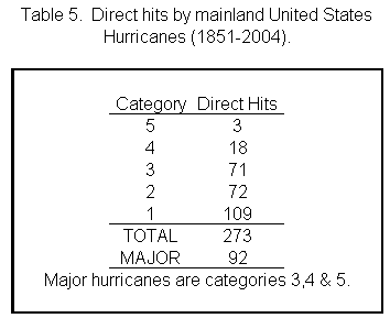
Exercise 2.1 Consider the following relative frequency table on hurricanes that have made direct hits on the U.S. between 1851 and 2004 (http://www.nhc.noaa.gov/gifs/table5.gif). Hurricanes are given a strength category rating based on the minimum wind speed generated by the storm. Some of the entries to the table are missing.

Frequency of Hurricane Direct Hits
Category	# Direct Hits	Relative Freq.	Cum. Relative Freq.
1	109
2	72	0.2637	0.6630
3		0.2601
4	18		0.9890
5	3	0.0110	1.0000

What is the relative frequency of direct hits of category 1?
What is the relative frequency of direct hits of category 4 or more?

Exercise 2.2 The number of calves that were born to some cows during their productive years was recorded. The data was entered into an R object by the name “calves”. Refer to the following R code:

freq <- table(calves)
cumsum(freq)

##  1  2  3  4  5  6  7 
##  4  7 18 28 32 38 45

How many cows were involved in this study?
How many cows gave birth to a total of 4 calves?
What is the relative frequency of cows that gave birth to at least 4 calves?

```

2.5 Summary

Glossary

Population:: The collection, or set, of all individuals, objects, or measurements whose properties are being studied.
Sample:: A portion of the population understudy. A sample is representative if it characterizes the population being studied.
Frequency:: The number of times a value occurs in the data.
Relative Frequency:: The ratio between the frequency and the size of data.
Cumulative Relative Frequency:: The term applies to an ordered set of data values from smallest to largest. The cumulative relative frequency is the sum of the relative frequencies for all values that are less than or equal to the given value.
Data Frame:: A tabular format for storing statistical data. Columns correspond to variables and rows correspond to observations.
Variable:: A measurement that may be carried out over a collection of subjects. The outcome of the measurement may be numerical, which produces a quantitative variable; or it may be non-numeric, in which case a factor is produced.
Observation:: The evaluation of a variable (or variables) for a given subject.
CSV Files:: A digital format for storing data frames.
Factor:: Qualitative data that is associated with categorization or the description of an attribute.
Quantitative:: Data generated by numerical measurements.

`R` functions introduced in this chapter

data.frame() creates data frames, tightly coupled collections of variables which share many of the properties of matrices and of lists, used as the fundamental data structure by most of R’s modeling software.
head() and tail() return the first or last parts of a data.frame.
sum() and cumsum() returns the sum and cumulative sum of the values present in its arguments.
read.csv(file) reads a file in table format and creates a data frame from it.

Discuss in the forum

Factors are qualitative data that are associated with categorization or the description of an attribute. On the other hand, numeric data are generated by numerical measurements. A common practice is to code the levels of factors using numerical values. What do you think of this practice?

In the formulation of your answer to the question you may think of an example of factor variable from your own field of interest. You may describe a benefit or a disadvantage that results from the use of a numerical values to code the level of this factor.

If the file is located in a different directory than the complete address, including the path to the file, should be provided. The file need not reside on the computer. One may provide, for example, a URL (an internet address) as the address. Thus, instead of saving the file of the example on the computer one may read its content into an R object by using the line of code “ex.1 <- read.csv(http://pluto.huji.ac.il/~msby/StatThink/Datasets/ex1.csv)” instead of the code that we provide and the working method that we recommend to follow.↩