Chapter 15 A Bernoulli Response

15.1 Student Learning Objectives

Chapters 13 and 14 introduced statistical inference that involves a response and an explanatory variable that may affect the distribution of the response. In both chapters the response was numeric. The two chapters differed in the data type of the explanatory variable. In Chapter 13 the explanatory variable was a factor with two levels that splits the sample into two sub-samples. In Chapter 14 the explanatory variable was numeric and produced, together with the response, a linear trend. The aim in this chapter is to consider the case where the response is a Bernoulli variable. Such a variable may emerge as the indicator of the occurrence of an event associated with the response or as a factor with two levels. The explanatory variable is a factor with two levels in one case or a numerical variable in the other case.

Specifically, when the explanatory variable is a factor with two levels then we may use the function “prop.test”. This function was used in Chapter 12 for the analysis of the probability of an event in a single sample. Here we use it in order to compare between two sub-samples. This is similar to the way the function “t.test” was used for a numeric response for both a single sample and for the comparison between sub-samples. For the case where the explanatory variable is numeric we may use the function “glm”, acronym for Generalized Linear Model, in order to fit an appropriate regression model to the data.

By the end of this chapter, the student should be able to:

Produce mosaic plots of the response and the explanatory variable.
Apply the function “prop.test” in order to compare the probability of an event between two sub-populations
Define the logistic regression model that relates the probability of an event in the response to a numeric explanatory variable.
Fit the logistic regression model to data using the function “glm” and produce statistical inference on the fitted model.

15.2 Comparing Sample Proportions

In this chapter we deal with a Bernoulli response. Such a response has two levels, “TRUE” or “FALSE”⁸², and may emerges as the indicator of an event. Else, it may be associated with a factor with two levels and correspond to the indication of one of the two levels. Such response was considered in Chapters 11 and 12 where confidence intervals and tests for the probability of an event where discussed in the context of a single sample. In this chapter we discuss the investigation of relations between a response of this form and an explanatory variable.

We start with the case where the explanatory variable is a factor that has two levels. These levels correspond to two sub-populations (or two settings). The aim of the analysis is to compare between the two sub-populations (or between the two settings) the probability of the even.

The discussion in this section is parallel to the discussion in Section 13.3. That section considered the comparison of the expectation of a numerical response between two sub-populations. We denoted these sub-populations \(a\) and \(b\) with expectations \(\Expec(X_a)\) and \(\Expec(X_b)\), respectively. The inference used the average \(\bar X_a\), which was based on a sub-sample of size \(n_a\), and the average \(\bar X_b\), which was based on the other sub-sample of size \(n_b\). The sub-samples variances \(S^2_a\) and \(S^2_b\) participated in the inference as well. The application of a test for the equality of the expectations and a confidence interval where produced by the application of the function “t.test” to the data.

The inference problem, which is considered in this chapter, involves an event. This event is being examined in two different settings that correspond to two different sub-population \(a\) and \(b\). Denote the probabilities of the event in each of the sub-populations by \(p_a\) and \(p_b\). Our concern is the statistical inference associated with the comparison of these two probabilities to each other.

Natural estimators of the probabilities are \(\hat P_a\) and \(\hat P_b\), the sub-samples proportions of occurrence of the event. These estimators are used in order to carry out the inference. Specifically, we consider here the construction of a confidence interval for the difference \(p_a - p_b\) and a test of the hypothesis that the probabilities are equal.

The methods for producing the confidence intervals for the difference and for testing the null hypothesis that the difference is equal to zero are similar is principle to the methods that were described in Section \[sec:TwoSamp\_3\] for making parallel inferences regarding the relations between expectations. However, the derivations of the tools that are used in the current situation are not identical to the derivations of the tools that were used there. The main differences between the two cases is the replacement of the sub-sample averages by the sub-sample proportions, a difference in the way the standard deviation of the statistics are estimated, and the application of a continuity correction. We do not discuss in this chapter the theoretical details associated with the derivations. Instead, we demonstrate the application of the inference in an example.

The variable “num.of.doors” in the data frame “cars” describes the number of doors a car has. This variable is a factor with two levels, “two” and “four”. We treat this variable as a response and investigate its relation to explanatory variables. In this section the explanatory variable is a factor with two levels and in the next section it is a numeric variable. Specifically, in this section we use the factor “fuel.type” as the explanatory variable. Recall that this variable identified the type of fuel, diesel or gas, that the car uses. The aim of the analysis is to compare the proportion of cars with four doors between cars that run on diesel and cars that run on gas.

Let us first summarize the data in a \(2 \times 2\) frequency table. The function “table” may be used in order to produce such a table:

cars <- read.csv("_data/cars.csv")
table(cars$fuel.type,cars$num.of.doors)

##         
##          four two
##   diesel   16   3
##   gas      98  86

When the function “table” is applied to a combination of two factors then the output is a table of joint frequencies. Each entry in the table contains the frequency in the sample of the combination of levels, one from each variable, that is associated with the entry. For example, there are 16 cars in the data set that have the level “four” for the variable “num.of.doors” and the level “diesel” for the variable “fuel.type”. Likewise, there are 3 cars that are associated with the combination “two” and “diesel”. The total number of entries to the table is \(16 + 3 + 98 + 86 = 203\), which is the number of cars in the data set, minus the two missing values in the variable “num.of.doors”.

A graphical representation of the relation between the two factors can be obtained using a mosaic plot. This plot is produced when the input to the function “plot” is a formula where both the response and the explanatory variables are factors:

plot(num.of.doors ~ fuel.type,data=cars)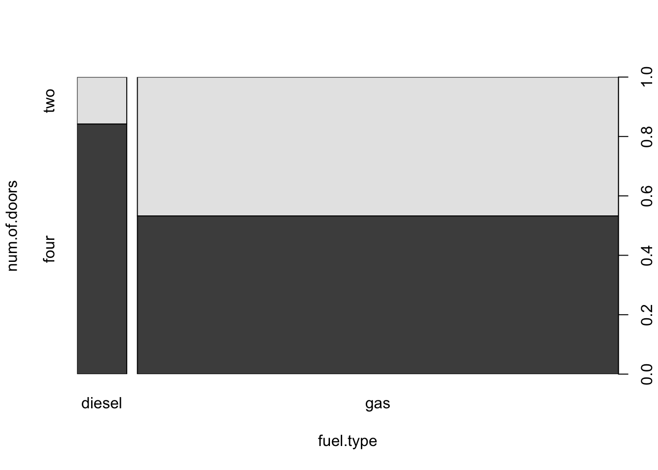

FIGURE 15.1: Number of Doors versus Fuel Type

The box plot describes the distribution of the explanatory variable and the distribution of the response for each level of the explanatory variable. In the current example the explanatory variable is the factor “fuel” that has 2 levels. The two levels of this variable, “diesel” and “gas”, are given at the \(x\)-axis. A vertical rectangle is associated with each level. These 2 rectangles split the total area of the square. The total area of the square represents the total relative frequency (which is equal to 1). Consequently, the area of each rectangle represents the relative frequency of the associated level of the explanatory factor.

A rectangle associated with a given level of the explanatory variable is further divided into horizontal sub-rectangles that are associated with the response factor. In the current example each darker rectangle is associated with the level “four” of the response “num.of.door” and each brighter rectangle is associated with the level “two”. The relative area of the horizontal rectangles within each vertical rectangle represent the relative frequency of the levels of the response within each subset associated with the level of the explanatory variable.

Looking at the plot one may appreciate the fact that diesel cars are less frequent than cars that run on gas. The graph also displays the fact that the relative frequency of cars with four doors among diesel cars is larger than the relative frequency of four doors cars among cars that run on gas.

The function “prop.test” may be used in order test the hypothesis that, at the population level, the probability of the level “four” of the response within the sub-population of diesel cars (the height of the leftmost darker rectangle in the theoretic mosaic plot that is produced for the entire population) is equal to the probability of the same level of the response with in the sub-population of cars that run on gas (the height of the rightmost darker rectangle in that theoretic mosaic plot). Specifically, let us test the hypothesis that the two probabilities of the level “four”, one for diesel cars and one for cars that run on gas, are equal to each other.

The output of the function “table” may serve as the input to the function “prop.test”⁸³. The Bernoulli response variable should be the second variable in the input to the table whereas the explanatory factor is the first variable in the table. When we apply the test to the data we get the report:

prop.test(table(cars$fuel.type,cars$num.of.doors))

## 
##  2-sample test for equality of proportions with continuity
##  correction
## 
## data:  table(cars$fuel.type, cars$num.of.doors)
## X-squared = 5.5021, df = 1, p-value = 0.01899
## alternative hypothesis: two.sided
## 95 percent confidence interval:
##  0.1013542 0.5176389
## sample estimates:
##    prop 1    prop 2 
## 0.8421053 0.5326087

The two sample proportions of cars with four doors among diesel and gas cars are presented at the bottom of the report and serve as estimates of the sub-populations probabilities. Indeed, the relative frequency of cars with four doors among diesel cars is equal to \(\hat p_a = 16/(16+3) = 16/19 = 0.8421053\). Likewise, the relative frequency of cars with four doors among cars that ran on gas is equal to \(\hat p_b = 98/(98+86) = 98/184 = 0.5326087\). The confidence interval for the difference in the probability of a car with four doors between the two sub-populations, \(p_a - p_b\), is reported under the title “95 percent confidence interval” and is given as \([0.1013542, 0.5176389]\).

The null hypothesis, which is the subject of this test, is \(H_0: p_a = p_b\). This hypothesis is tested against the two-sided alternative hypothesis \(H_1: p_a \not = p_b\). The test itself is based on a test statistic that obtains the value X-squared = 5.5021. This test statistic corresponds essentially to the deviation between the estimated value of the parameter (the difference in sub-sample proportions of the event) and the theoretical value of the parameter (\(p_a - p_b = 0\)). This deviation is divided by the estimated standard deviation and the ratio is squared. The statistic itself is produced via a continuity correction that makes its null distribution closer to the limiting chi-square distribution on one degree of freedom. The \(p\)-value is computed based on this limiting chi-square distribution.

Notice that the computed \(p\)-value is equal to p-value = 0.01899. This value is smaller than 0.05. Consequently, the null hypothesis is rejected at the 5% significance level in favor of the alternative hypothesis. This alternative hypothesis states that the sub-populations probabilities are different from each other.

15.3 Logistic Regression

In the previous section we considered a Bernoulli response and a factor with two levels as an explanatory variable. In this section we use a numeric variable as the explanatory variable. The discussion in this section is parallel to the discussion in Chapter \[ch:Regression\] that presented the topic of linear regression. However, since the response is not of the same form, it is the indicator of a level of a factor and not a regular numeric response, then the tools the are used are different. Instead of using linear regression we use another type of regression that is called Logistic Regression.

Recall that linear regression involved fitting a straight line to the scatter plot of data points. This line corresponds to the expectation of the response as a function of the explanatory variable. The estimated coefficients of this line are computed from the data and used for inference.

In logistic regression, instead of the consideration of the expectation of a numerical response, one considers the probability of an event associated with the response. This probability is treated as a function of the explanatory variable. Parameters that determine this function are estimated from the data and are used for inference regarding the relation between the explanatory variable and the response. Again, we do not discuss the theoretical details involved in the derivation of logistic regression. Instead, we apply the method to an example.

We consider the factor “num.of.doors” as the response and the probability of a car with four doors as the probability of the response. The length of the car will serve as the explanatory variable. Measurements of lengths of the cars are stored in the variable “length” in the data frame “cars”.

First, let us plot the relation between the response and the explanatory variable:

plot(num.of.doors ~ length,data=cars)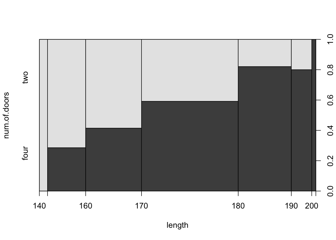

FIGURE 15.2: Number of Doors versus Fuel Type

The plot is a type of a mosaic plot and it is produced when the input to the function “plot” is a formula with a factor as a response and a numeric variable as the explanatory variable. The plot presents, for interval levels of the explanatory variable, the relative frequencies of each interval. It also presents the relative frequency of the levels of the response within each interval level of the explanatory variable.

In order to get a better understanding of the meaning of the given mosaic plot one may consider the histogram of the explanatory variable.

hist(cars$length)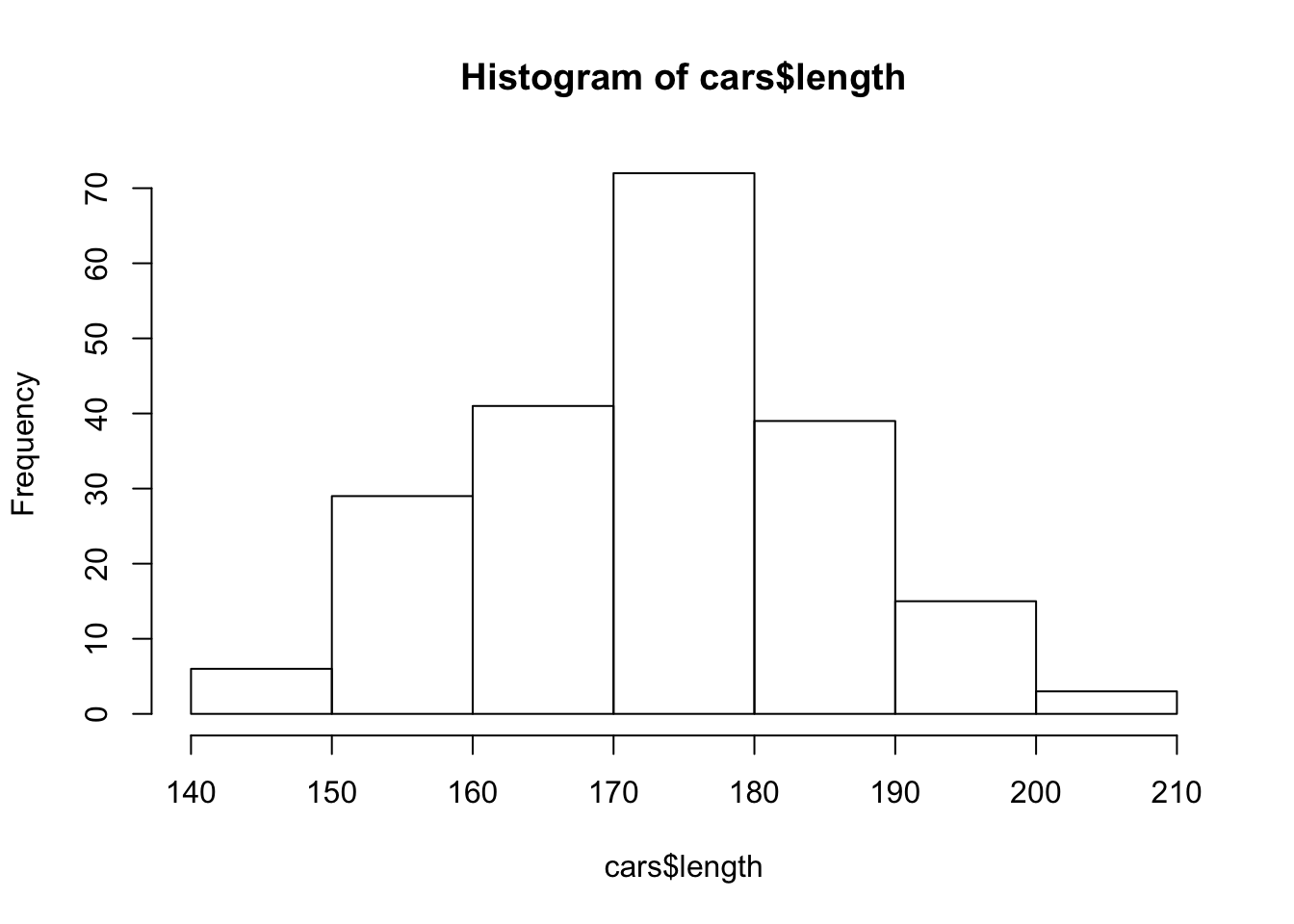

FIGURE 15.3: Histogram of the Length of Cars

The histogram involves the partition of the range of variable length into intervals. These interval are the basis for rectangles. The height of the rectangles represent the frequency of cars with lengths that fall in the given interval.

The mosaic plot in Figure 15.2 is constructed on the basis of this histogram. The \(x\)-axis in this plot corresponds to the explanatory variable “length”. The total area of the square in the plot is divided between 7 vertical rectangles. These vertical rectangles correspond to the 7 rectangles in the histogram of Figure 15.3, turn on their sides. Hence, the width of each rectangle in Figure 15.2 correspond to the hight of the parallel rectangle in the histogram. Consequently, the area of the vertical rectangles in the mosaic plot represents the relative frequency of the associated interval of values of the explanatory variable.

The rectangle that is associated with each interval of values of the explanatory variable is further divided into horizontal sub-rectangles that are associated with the response factor. In the current example each darker rectangle is associated with the level “four” of the response “num.of.door” and each brighter rectangle is associated with the level “two”. The relative area of the horizontal rectangles within each vertical rectangle represent the relative frequency of the levels of the response within each interval of values of the explanatory variable.

From the examination of the mosaic plot one may identify relations between the explanatory variable and the relative frequency of an identified level of the response. In the current example one may observe that the relative frequency of the cars with four doors is, overall, increasing with the increase in the length of cars.

Logistic regression is a method for the investigation of relations between the probability of an event and explanatory variables. Specifically, we use it here for making inference on the number of doors as a response and the length of the car as the explanatory variable.

Statistical inference requires a statistical model. The statistical model in logistic regression relates the probability \(p_i\), the probability of the event for observation \(i\), to \(x_i\), the value of the response for that observation. The relation between the two in given by the formula:

\[p_i = \frac{e^{a + b \cdot x_i}}{1 + e^{a + b\cdot x_i}}\;,\] where \(a\) and \(b\) are coefficients common to all observations. Equivalently, one may write the same relation in the form:

\[\log(p_i/[1-p_i]) = a + b\cdot x_i\;,\] that states that the relation between a (function of) the probability of the event and the explanatory variable is a linear trend.

One may fit the logistic regression to the data and test the null hypothesis by the use of the function “glm”:

fit.doors <- glm(num.of.doors=="four"~length, family=binomial,data=cars)
summary(fit.doors)

## 
## Call:
## glm(formula = num.of.doors == "four" ~ length, family = binomial, 
##     data = cars)
## 
## Deviance Residuals: 
##     Min       1Q   Median       3Q      Max  
## -2.1646  -1.1292   0.5688   1.0240   1.6673  
## 
## Coefficients:
##              Estimate Std. Error z value Pr(>|z|)    
## (Intercept) -13.14767    2.58693  -5.082 3.73e-07 ***
## length        0.07726    0.01495   5.168 2.37e-07 ***
## ---
## Signif. codes:  0 '***' 0.001 '**' 0.01 '*' 0.05 '.' 0.1 ' ' 1
## 
## (Dispersion parameter for binomial family taken to be 1)
## 
##     Null deviance: 278.33  on 202  degrees of freedom
## Residual deviance: 243.96  on 201  degrees of freedom
##   (2 observations deleted due to missingness)
## AIC: 247.96
## 
## Number of Fisher Scoring iterations: 3

Generally, the function “glm” can be used in order to fit regression models in cases where the distribution of the response has special forms. Specifically, when the argument “family=binomial” is used then the model that is being used in the model of logistic regression. The formula that is used in the function involves a response and an explanatory variable. The response may be a sequence with logical “TRUE” or “FALSE” values as in the example⁸⁴. Alternatively, it may be a sequence with “1” or “0” values, “1” corresponding to the event occurring to the subject and “0” corresponding to the event not occurring. The argument “data=cars” is used in order to inform the function that the variables are located in the given data frame.

The “glm” function is applied to the data and the fitted model is stored in the object “fit.doors”.

A report is produced when the function “summary” is applied to the fitted model. Notice the similarities and the differences between the report presented here and the reports for linear regression that are presented in Chapter 14. Both reports contain estimates of the coefficients \(a\) and \(b\) and tests for the equality of these coefficients to zero. When the coefficient \(b\), the coefficient that represents the slope, is equal to 0 then the probability of the event and the explanatory variable are unrelated. In the current case we may note that the null hypothesis \(H_0: b = 0\), the hypothesis that claims that there is no relation between the explanatory variable and the response, is clearly rejected (\(p\)-value \(2.37 \times 10^{-7}\)).

The estimated values of the coefficients are \(-13.14767\) for the intercept \(a\) and \(0.07726\) for the slope \(b\). One may produce confidence intervals for these coefficients by the application of the function “confint” to the fitted model:

confint(fit.doors)

## Waiting for profiling to be done...

##                    2.5 %     97.5 %
## (Intercept) -18.50384373 -8.3180877
## length        0.04938358  0.1082429

15.4 Exercises

Exercise 15.1 This exercise deals with a comparison between Mediterranean diet and low-fat diet recommended by the American Heart Association in the context of risks for illness or death among patients that survived a heart attack⁸⁵. This case study is taken from the Rice Virtual Lab in Statistics. More details on this case study can be found in the case study “Mediterranean Diet and Health” that is presented in that site.

The subjects, 605 survivors of a heart attack, were randomly assigned follow either (1) a diet close to the “prudent diet step 1” of the American Heart Association (AHA) or (2) a Mediterranean-type diet consisting of more bread and cereals, more fresh fruit and vegetables, more grains, more fish, fewer delicatessen food, less meat.

The subjects‘ diet and health condition were monitored over a period of four-year. Information regarding deaths, development of cancer or the development of non-fatal illnesses was collected. The information from this study is stored in the file “diet.csv”. The file “diet.csv” contains two factors: “health” that describes the condition of the subject, either healthy, suffering from a non-fatal illness, suffering from cancer, or dead; and the “type” that describes the type of diet, either Mediterranean or the diet recommended by the AHA. The file can be found on the internet at http://pluto.huji.ac.il/~msby/StatThink/Datasets/diet.csv. Answer the following questions based on the data in the file:

Produce a frequency table of the two variable. Read off from the table the number of healthy subjects that are using the Mediterranean diet and the number of healthy subjects that are using the diet recommended by the AHA.
Test the null hypothesis that the probability of keeping healthy following an heart attack is the same for those that use the Mediterranean diet and for those that use the diet recommended by the AHA. Use a two-sided alternative and a 5% significance level.
Compute a 95% confidence interval for the difference between the two probabilities of keeping healthy.

Exercise 15.2 Cushing’s syndrome disorder results from a tumor (adenoma) in the pituitary gland that causes the production of high levels of cortisol. The symptoms of the syndrome are the consequence of the elevated levels of this steroid hormone in the blood. The syndrome was first described by Harvey Cushing in 1932.

The file “coshings.csv" contains information on 27 patients that suffer from Cushing’s syndrome⁸⁶. The three variables in the file are “tetra”, “pregn”, and “type”. The factor “type” describes the underlying type of syndrome, coded as “a“, (adenoma),”b" (bilateral hyperplasia), “c” (carcinoma) or “u” for unknown. The variable “tetra” describe the level of urinary excretion rate (mg/24hr) of Tetrahydrocortisone, a type of steroid, and the variable “pregn” describes urinary excretion rate (mg/24hr) of Pregnanetriol, another type of steroid. The file can be found on the internet at http://pluto.huji.ac.il/~msby/StatThink/Datasets/coshings.csv. Answer the following questions based on the information in this file:

Plot the histogram of the variable “tetra” and the mosaic plot that describes the relation between the variable “type” as a response and the variable “tetra”. What is the information that is conveyed by the second vertical triangle from the right (the third from the left) in the mosaic plot.
Test the null hypothesis that there is no relation between the variable “tetra” as an explanatory variable and the indicator of the type being equal to “b” as a response. Compute a confidence interval for the parameter that describes the relation.
Repeat the analysis from 2 using only the observations for which the type is known. (Hint: you may fit the model to the required subset by the inclusion of the argument “subset=(type!=u)” in the function that fits the model.) Which of the analysis do you think is more appropriate?

Glossary

Mosaic Plot:: A plot that describes the relation between a response factor and an explanatory variable. Vertical rectangles represent the distribution of the explanatory variable. Horizontal rectangles within the vertical ones represent the distribution of the response.
Logistic Regression:: A type of regression that relates between an explanatory variable and a response of the form of an indicator of an event.

Discuss in the forum

In the description of the statistical models that relate one variable to the other we used terms that suggest a causality relation. One variable was called the “explanatory variable” and the other was called the “response”. One may get the impression that the explanatory variable is the cause for the statistical behavior of the response. In negation to this interpretation, some say that all that statistics does is to examine the joint distribution of the variables, but casuality cannot be inferred from the fact that two variables are statistically related. What do you think? Can statistical reasoning be used in the determination of casuality?

As part of your answer in may be useful to consider a specific situation where the determination of casuality is required. Can any of the tools that were discussed in the book be used in a meaningful way to aid in the process of such determination?

Notice that the last 3 chapters dealt with statistical models that related an explanatory variable to a response. We considered tools that can be used when both variable are factors and when both are numeric. Other tools may be used when one of the variables is a factor and the other is numeric. An analysis that involves one variable as the response and the other as explanatory variable can be reversed, possibly using a different statistical tool, with the roles of the variables exchanged. Usually, a significant statistical finding will be still significant when the roles of a response and an explanatory variable are reversed.

Formulas:

Logistic Regression, (Probability): \(p_i = \frac{e^{a + b \cdot x_i}}{1 + e^{a + b\cdot x_i}}\).
Logistic Regression, (Predictor): \(\log(p_i/[1-p_i]) = a + b\cdot x_i\).

The levels are frequently coded as 1 or 0, “success” or “failure”, or any other pair of levels.↩
The function “prop.test” was applied in Section 12.4 in order to test that the probability of an event is equal to a given value (“p = 0.5” by default). The input to the function was a pair of numbers: the total number of successes and the sample size. In the current application the input is a \(2 \times 2\) table. When applied to such input the function carries out a test of the equality of the probability of the first column between the rows of the table.↩
The response is the output of the expression “num.of.doors==four”. This expression produces logical values. “TRUE” when the car has 4 doors and “FALSE” when it has 2 doors.↩
De Lorgeril, M., Salen, P., Martin, J., Monjaud, I., Boucher, P., Mamelle, N. (1998). Mediterranean Dietary pattern in a Randomized Trial. Archives of Internal Medicine, 158, 1181-1187.↩
The source of the data is the data file “Cushings” from the package “MASS” in R.↩